Linear Shaping of Signals | RC(LR) & CR(RL) circuits

When simple periodic (sinusoidal) signals are applied on the electric circuits which contains linear R, L, C elements, then the response of these circuits in stationary mode is proportional to the input signal. The effect of these circuits on the input signal is expressed only with the relationship of the amplitudes or the phases of the input and output signal, but the shape of the signal is preserved. Therefore, these kind of circuits are called linear electric circuits. However, the response of these circuits for complex, not-simple periodic signal, will undergo change not only in the amplitude of the signal, but also in its shape, due to the unequal impact of the circuits on the harmonic components contained in the input signal. The process of changing the shape of the signals through these kind of linear circuits is called linear shaping of signals.

In the pulse electronics, the not-simple periodic signals are exactly of great importance. These signals are so called pulse signals and they are characterized with step change in their amplitude. Examples of pulse signals are: rectangular pulses, linear increasing/decreasing signals, exponentional signals, aperiodic pulse signals with complex shape, and so on.

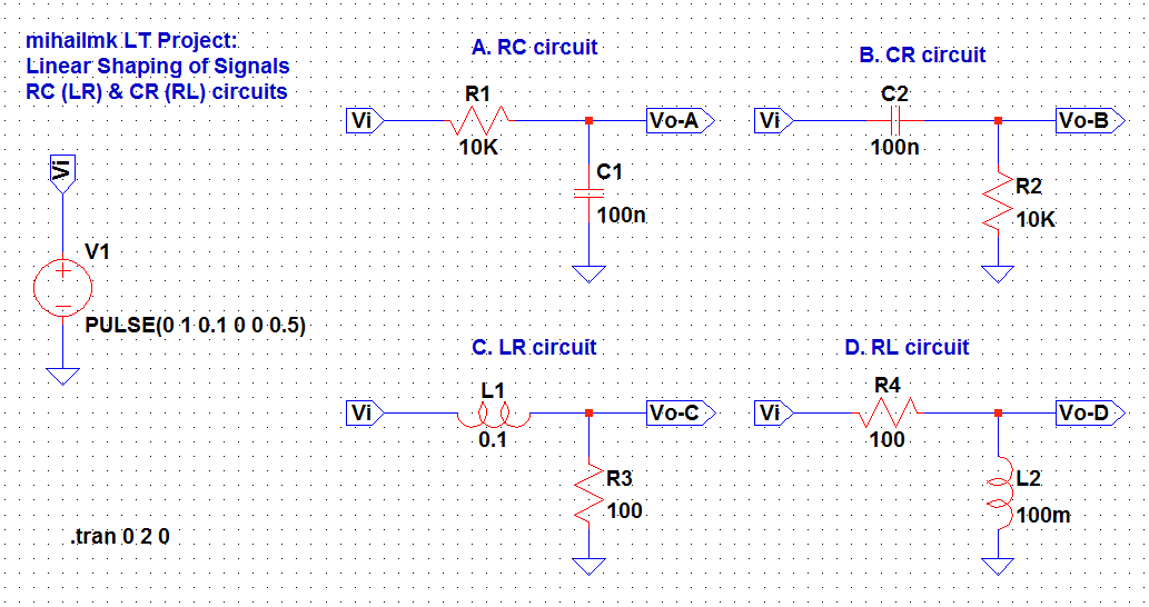
Picture 1: Simple RC(LR) & CR(RL) circuits for Linear Shaping of Signals


On Picture 1 are shown simple examples of RC(LR) and CR(RL) circuits. Because of the way of which these circuits impact on the harmonics from the spectrum of the input signal, they are called low-pass or high-pass circuits. According to the function of these circuits, the circuit A. (RC circuit) is equivalent to the circuit C. (LR circuit) and the circuit B. (CR circuit) is equivalent to the circuit D. (RL circuit), if the relation RC = L/R is satisfied.

The analysis of these circuits is based on the energy state of the energy storage elements, capacitor C and inductor L, that can be expressed via the dynamic equations which describes the physical nature of these elements. In other words, the voltage of the capacitor ends through which flows final current, can not have an discontinuous change, or it must apply that Vc(t+) = Vc(t-). The current that flows through inductor coil which is exposed on the final voltage on its ends, can not have an step change, or it must apply that iL(t+) = iL(t-).

If a step-voltage is applied on the input of linear RC circuit, then the response of the circuit will follow some shape from starting value to final value of the output signal. In theory, the final value of the output voltage will be achieved after infinitely long time. However, in practice, the 95% of the final value is achieved after the period of time t = 3τ, where τ = RC is the time constant of the circuit. This time is considered sufficient for achieving the stationary (steady) state of the circuit.

In many applications of great importance is the time duration of the front, or rear edge of the signal, the so called rise-time, or fall-time, which is defined as time needed for change in the amplitude of the signal from 10% up to 90% of its final value.

Time-domain analysis

Now, let's see the results of the transient analysis for these 4 linear circuits in time domain. We choose to analyze the response of these circuits for the rectangular pulse as input signal. Therefore, we set the independent voltage source V1 as pulse generator, to generate the rectangular pulse with amplitude of 1 V and time duration of 0.5 seconds. The delay time period for this pulse is set to 100 ms, and the rise-time and fall-time are set to zero. The input voltage wave form is shown on Picture 2. Although we set the rise and fall time of the pulse to zero, as we can see from the plot, it takes of about 50 ms for the pulse to achieve the value of 1 V and fall back to zero volts again.

Picture 2: Input voltage wave form (time-domain)


Furthermore, as we can see from the circuit elements shown on Picture 1, we chose the values of 100 nF and 10 kOhms for the CR and RC circuits, so their time constant is equal to τ = RC = 1 ms. Also, for the LR and RL circuits we choose values of 100 mH and 100 ohms, so their time constant is also τ = L/R = 1 ms. Thus, we have satisfied the condition RC = L/R, so the A. and C. circuits are equivalent, and B. and D. circuits are also equivalent.

Picture 3: Output voltage wave forms of the A. RC circuit & C. LR circuit (time-domain)


The wave forms of the output voltages Vo-A and Vo-C are shown on Picture 3. As we can see, both plots match to eachother as expected from the condition of equal time constants. Furthermore, they match the input voltage signal, so we can say that these two circuits A. and C. do not affect the input signal at all, since they didn't change its shape, nor it's amplitude.

Picture 4: Output voltage wave forms of the B. CR circuit & D. RL circuit (time-domain)


From the other hand, the circuits B. and D. have changed the shape of the input signal, as we can see from Picture 4. The wave forms of the output voltages Vo-B and Vo-D are both same, as expected. We can notice that these ouput signals consists of two rectangular pulses. The first of them is positive with amplitude of +20 mV and time duration of about 50 ms, which match the timing of rising of the input signal, and the second pulse is negative with amplitude of -20 mV and same duration of about 50 ms, which match the timing of falling of the input signal from 1 to 0 volts.