Setting rules for PID Controller

Setting rules to Ziegler/Nichols

Right at the initial stage of modern control technology, J.G. Ziegler and N.B. Nichols have specified setting rules (Picture 1), which are still widely used today. These are intended for cases where no model (or inflectional tangent model) of the controlled system is available and the closed control loop can be operated safely along the stability limit.

These rules are as follows:

1. Set the controller as a P-controller (Tv = 0 Tn = ...).
2. The amplitude factor KR of the controller is increased until the closed control loop is on the point of performing unattenuated oscillations (stability limit). This determines the critical amplitude factor KRk and the period of oscillation Tk of this sustained oscillation.
3. Based on these two parameters (KRk, Tk), the controller parameters KR, Tn and Tv are then to be calculated as per controller type according to the following specification and set on the computer.

Picture 1: Setting rules to Ziegler/Nichols


However, experience shows that these setting values only lead to workable closed control loop behaviour, if the ratio of transient time Tg to time delay Tu of the controlled system is not too great, i.e. the system in the model of the transient function shows a noticeable time delay.

Setting rules to Chien/Hrones/Reswick

If we are dealing with an inflectional tangent model of the controlled system, then the setting rules of Chien, Hrones and Reswick are to be used. The setting rules for this are shown in the following table (Picture 2).

Picture 2: Setting rules to Chien/Hrones/Reswick


For I-controlled systems the expression:

1/(KIS * Tu)

is to be used instead of:

Tg/(KS * Tu).

These rules can also be applied to a total time constant model, provided Tu = Tt and Tg = T are set.

Function mode of Operation of Technical Controllers

Control algorithms

Control algorithms have proved to be a tried and tested method of calculating the correcting variable Y from the system deviation e, which relates back to the basic behaviour patterns of the response characteristic (P-, I-, D-action) of technical systems. Each action assumes its own particular role in the course of this processing of information. Picture 1 shows the signal flow diagram (the graphic representation of signal processing) of the controller. The purpose of P and D-action is to ensure an as quick as possible but smooth process of the transient phenomenon in closed control loops. The D-action does not have any effect on the stationary state of a closed control loop, since even with a steady-state deviation es (τµ) 0, the output signal YD decays towards zero and therefore does not contribute towards the stationary value of the control signal Y. However, the effect of this action comes into force particularly quickly with variable system deviations. To some degree, the D-action therefore contributes in advance, i.e. in anticipatory manner to the control signal Y. The actual action function is to keep the controller characteristic curve vertical and thus to completely correct any permanent interference. This relates to the previously illustrated characteristic of integral-action systems to generate a constant rate of change of the system output variable after a jump activation. This is how the system output (in the case of the controller, the signal Y) can assume any I value within its control range, even though the input signal (in this case the system deviation e) attains the value zero again after a transient response. An integral action system therefore has a steady-state effect in the same way as a proportionally acting system with infinitely significant proportional coefficient. Over a sufficiently long period of time, the smallest uni-dimensional input signal values lead to an output signal of some significance. In order to be able to calculate the overall effect of the controller on the closed control loop behaviour and as such the time-related response of controlled variables X and Y in relation to the task, the controller actions can be introduced into the calculation of the values of setpoint specification Y. For this, every PID controllers has three freely adjustable parameters (characteristic controller values):

>> the proportional coefficient KR for the adjustment of the P-action;
>> the correction time Tn for the adjustment of the I-action;
>> the derivative-action time Tv for the adjustment of the D-action.

Dynamic closed control loop behaviour requirements

The adjustment of the characteristic controller values KR, Tn and Tv largely depends on:

>> the steady-state and dynamic behaviour of the controlled system;
>> the disturbances acting on the controlled system;
>> the demands placed on the steady-state and dynamic behaviour of the closed control loop.

The steady-state behaviour of the closed control loop (working point setting, steady-state system deviation, functions and effect of the I-action in the controller) has already been described in detail in the section Steady-state behaviour of the closed control loop in Controller Configuration and Parameterisation.

Picture 1: Signal flow diagram of PID-controller:
a) with individual representation of controller actions P, I and D
b) with overall representation (Addition of individual representations) of controller transient function hR(t)


The same preconditions should be assumed for the discussion of the dynamic behaviour as those applied for the linear dynamic model of technical systems. Here, it is assumed that all process signals during the control processes occur in the vicinity of their working points and do not in practice deviate from the linearity range. In this way, the demands placed on the dynamic behaviour of the closed control loop, e. g. in the form of step responses can be precisely defined. However, this means that during the practical operation of the closed control loop, the boundaries of the linear working range around the working point must be observed. If these are exceeded, then the results achievable in this case with the controller settings based on the linear dynamic models are also called into question.

Picture 2 illustrates a behaviour of the controlled variable x(t) after the sudden change of the setpoint value w (control step response of the closed control loop), which should be aimed for. This behaviour can be described roughly by two characteristic values:

>> the overshoot time Tm;
>> the standardised overshoot amplitude ∆h = ∆h∗ / w.

The overshoot amplitude ∆h usually requires a value between 0 and 20 %t. Overshoot time requirements Tm depend on the dynamic behaviour of the closed control loop and must always be viewed in conjunction with the process dead times and process constants. If the inflectional tangent model introduced in the section The inflectional tangent model in The Inflectional Tangent & The Total Time Constant model is used to describe the controlled system behaviour, then the overshoot time should not be less than half the total of the time delay and the transient time specified (reference value). This ensures that the control signal y does not assume untenably high values during the transient stage.

Picture 2: Favourable behaviour of control step response of a closed control loop


A similar process can be adopted with regard to a favourable course of the interference step response of the closed control loop (step-change response of the closed control loop at its input). Picture 3 shows a favourable course of this process from the control technology viewpoint.

Picture 3: Favourable behaviour of interference step response of a closed control loop


Here too, the process can be described roughly by means of two characteristic values (Tm and ∆h* or xm).

Controller Configuration and Parameterisation

Technical controllers are a component part of automation systems, whose main task is that of process stabilisation. They are used with the aim of:

>> bringing about and maintaining specific process states (mode of operation) automatically;
>> eliminating the effects of interference on the process sequence;
>> preventing unwanted coupling of part processes in the technical process.

The process states addressed primarily refer to specific process parameters, such as pressure, flow, temperature, filling level and quality (pH value).

Mode of operation of closed control loop

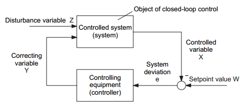
Picture 1 shows the basic structure of a closed control loop. Its mode of operation can be described as follows:

Picture 1: Mode of operation of closed control loop


The required value of the controlled variable X, i. e. its desired characteristic as a function of time, is specified by the setpoint value W. This can be done manually on the control equipment of the controller or also by a controlling device, which is of higher-order to the controller. In the case of a fixed setpoint value, we talk of a fixed setpoint control, and in the case of a time varying setpoint value of a setpoint control or servo control. The controlled variable X is continually measured via a suitable measuring device (or at permissible time intervals) and compared with the setpoint value W by means of subtraction.
The system deviation e = W - X indicates, how much and in which direction (e. g. valve to be opened or closed more) intervention in the process is necessary via the correcting variable Y in order to eliminate the occurring system deviation. The controlling device is used as an information processing system, which calculates the correcting variable Y appropriate for the control process from the existing system deviation.
Technical controlled systems are subject to a multitude of interference (load variations, changes in the quality of materials used, etc.). To simplify matters, Picture 1 therefore only includes one main disturbance variable Z. All disturbances have an effect on the controlled variable and change (e. g. in the case of a fixed setpoint control) its required operating point value Xo = Wo. As such, all disturbances are therefore reflected in the system deviation, and the above described control process, which is carried out continually and automatically, then ensures as complete a diminution of the system deviation as possible and thus the elimination of the effect of the disturbance on the controlled variable.
The success of a control system obviously depends critically on the time-related characteristic of the disturbance variables (and time varying setpoint values), the steady-state and dynamic behaviour of the controlled system and information processing in the controlling equipment.

Steady-state behaviour of the closed control loop

Similar to the deliberations regarding the simulation of the steady and dynamic behaviour of the technical system to be controlled (in this case controlled systems), it is also essential to discuss the concepts and descriptions regarding the steady-state and dynamic behaviour of closed control loops.
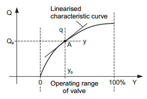
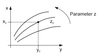
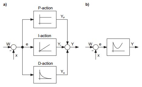
The description of the steady-state closed control loop behaviour again entails the use of characteristic curves or characteristics, in this case, the steady-state models of controlled system and controller. Hence Picture 2 (a) illustrates the steady-state characteristic of the controlled system and Picture 2 (b) the steady-state characteristic of a proportionally acting controller. Here, Y designates the correcting variable (e. g. valve position) and X the controlled variable (e. g. temperature).

Picture 2: Performance characteristic of: (a) controlled system (b) controlled device


Both characteristics can be represented jointly if identical scaling is selected (Picture 3). The interface between the valid characteristics for the controlled system (Z = Z0) and the controlling equipment (W = W0) result in the operating point Ao and hence the operating point values Y0 or X0 for the actuating signal Y or for the controlled variable signal X. If the interference then changes from Z = Z0 to Z = Z1, then, in the case if a fixed valve position Y0 (to remain with the example), i.e. with a controller which is switched off or has not been started up, the operating point would drift from A0 to A1 and the controlled variable X (e. g. the temperature) would assume the value X1 .

However, if the controller is active then, on the basis of the same considerations which apply to the interface A0, the operating point A2 occurs, since the now operative characteristic curves of the controlled system for Z= Z1 and of the controlling device for W = W0 (with unchanged setpoint value) now need to be intersected. The operating point in this case therefore drifts from A0 to A2. The corresponding operating point values are Y2 and X2. In order to prevent the unwanted increase of the controlled variable from X0 to X1 at least to some extent, the setpoint value is reset via the controller from Y0 to Y2 and the steady-state controlled variable value X2 set.
The flatter the form of the characteristic curve of the controller in Picture 3, the more effective the controller probably is with regard to the steady-state behaviour of the closed control loop. In the borderline case of a horizontally running controller characteristic curve, the control objective of complete diminution of the stationary system deviation es = W0 - X2, could even be completely achieved. However, a horizontally running controller characteristic curve as shown in Picture 3 means a vertical pattern in Picture 2 (b), and as such an infinitely high proportional coefficient of the controller assumed to be of proportional action. That this optimum steady-state closed control loop behaviour can actually be realised, can only be seen by further pursuing deliberation regarding information processing in technical controllers.

Picture 3: Steady-state performance characteristics of closed control loop, Interference changes from Z0 to Z1:
1. Working point variation with fixed setpoint value Y0
2. Working point variation with active closed-loop control

Model configuration for Temperature Control System

The temperature control system of the small-scale experimental modules in the experimental state consists of an electrically heatable container, in which the water temperature in increased (Picture 1). To obtain a better distribution of temperature in the container, the water can be agitated by means of a centrifugal pump. This results in constant thorough mixing, which prevents the formation of differing heat levels. The purpose of the automation task is to control the water temperature T (controlled variable) by means of the heat output Pel (correcting variable). The special characteristic of this controlled system is that the temperature is lowered solely as a result of heat dissipated to the environment. The output of this process, i. e. the heat dissipation ∆Qout in the time interval ∆t, is considerably less compared to the maximum heat output.

Picture 1: Schematic representation of temperature control system

The following abbreviations mean:

>> T - Water temperature in the container;
>> Tu - Ambient temperature (air);
>> ∆Qel - Quantity of heat output by heater system in ∆t;
>> ∆QL - Quantity of heat emitted directly to air in ∆t;
>> ∆QW - Quantity of heat emitted through wall in ∆t;
>> h - Filling level in container.

Theoretical model configuration

The heating process in the temperature control system can be represented in a greatly simplified manner as follows (Picture 2).

Picture 2: Simplified representation of temperature control system


The following mean:

>> V = c * m * T – internal energy of volume of water with m = ρV = ρ * A * h;
>> ∆Qel = Pel * ∆t – quantity of heat output via heating system in time interval ∆t;
>> ∆QL = α * AL * (T − Tu) * ∆t – quantity of heat (heat transmission) directly emitted to the air via the exposed water level in ∆t;
>> α – heat transmission coefficient (water – air);
>> ∆QW = k * AW * (T − Tu) * ∆t – quantity of heat (heat transmission) emitted to the air via the wall in ∆t;
>> k – heat transmission coefficient (water – container wall – air).


The quantity of heat supplied and removed during time interval ∆t, can be noted as follows:

∆Qin = Pel * ∆t       or

∆Qout = ∆QW + ∆QL

The temperature T only changes if a difference ∆Q occurs between the quantities of heat:

∆Q = ∆Qzu − ∆Qab

This difference is the change of the internal energy of the volume of water:

∆Q = ∆U = c * m * ∆T

Steady-state model of closed control loop

The supplied and removed quantities of heat must coincide in the stationary state (∆Q = const., ∆T = const.):

∆Qin = ∆Qout

and hence

Pel = α * AL * (T − Tu) + k * AW * (T − Tu)

must apply. With an assumed constant ambient temperature, this equation results in the correlation

T (Pel) = Pel/(α * AL + k * Aw) + Tu

which indicates the dependence between heating capacity output and water temperature in the stationary state. Picture 3 shows the steady-state characteristic curve of the temperature control system. An assumed constant ambient temperature becomes less and less valid with increased heat dissipation. With increasing ambient temperature, the lost heat flow decreases, (∆Qab ~ T-Tu), whereby the water temperature becomes higher than in the ideal case.


The heating module used can be actuated intermittently, since it is either switched on at full capacity or switched off completely (two-point element). Any desired heat output can be achieved by means of periodic switching on or off of the heating module. The periodic time tper is used to calculate the output from the switch-on time ton and the heat output in the switched on status Pelmax at:

Pel = Pel max * ton/tper

Picture 3: Qualitative process of steady-state characteristic curve of temperature control system (ideal case)


The periodic time tper must be sufficiently long so as not to excessively load the contactor in the control head in the heater modules as a result of frequent switching. On the other hand, the periodic time selected must be short, so that the temperature pattern remains even (Picture 4). This means that is must be considerably shorter than the controlled system time constant of the heating or cooling process (e. g. tper = 10 s).

Picture 4: Temperature and performance pattern during on/off switching of heater module (two-point element)

Linear dynamic controlled system model

If we now look at the following equation again:

∆Qin − ∆Qout = c * m * ∆T

and apply this for the supplied and dissipated quantity of heat, this results in the following correlation for the temperature change ∆T per time interval:

∆T/∆t = [1/(c * m)] * [Pel − (α * AL + k * AW) * (T − Tu)]

This controlled system section represents a sufficiently small ∆t selected, and is the basis of the behaviour shown in Picture 5 (a). The temperature control system therefore has a proportional action with a delay of the first order. The change in heat output causes a gradual temperature change.


Again, it should be pointed out that the rate of change in temperature is not the same for heating and cooling. Picture 5 shows the qualitative pattern of the two processes. In addition, a considerably shorter dead time Tt occurs in the case of heating compared to the system time constant THeating. This is caused by the heat capacity of the heater module and the heat conduction speed in the water. This latter time constant can be lowered by moving or stirring the water. The parameters K, THeating and TCooling are to be determined by experiment.

Picture 5: Qualitative representation of system step response: a) Heating b) Cooling

Model configuration for Filling Level Control System

The filling level control system in the experimental state consists of containers connected via two pipes and a pump, which are located at different height levels (see Picture 1). The water is conveyed from the lower to the upper container via the pump and pipe (1) and, from there, can freely flow back to the lower container again via pipe (2) by means of gravitational force. The purpose of the automation task is to regulate the water level in the upper container.

Picture 1: Schematic representation of level control system

Theoretical model configuration

Model for the outflowing process from the upper container

This outflowing process can be represented in a very simplified form (see Picture 2).

Picture 2: Physical model of outflow process


The following abbreviations mean:

>> p0 – Atmospheric pressure;
>> pB = p0 + ρgHH – Pressure at the bottom;
>> ∆p = kR2Qab^2 – Pressure drop via the pipe;
>> Qab – Volumetric flow rate;

and ∆p = pB - p0 = ρgHh

becomes the volumetric outward flow Qab = k * √ {ρgHH}

Dynamic processes in piping systems, which could lead to delays of the processes, are disregarded in this instance, since the dynamic behaviour is determined mainly by the storage processes in the two containers.

Model for inflow process into the upper container

On the basis of the same deliberations as already described in detail, a balance must again exist between the partial pressures in the system, for which the following applies:

0 = ∆p0 − ∆pstat − ∆pR − ∆pi

Using

∆pstat = ρg (HA + HH − HU)
∆pR = kR1Qin^2
∆pi = kiQin^2

results in the condition:

0 = kpN^2 − ρg (HA + HH − HU) − (ki + kR) Qin^2

Here it should be noted that if the containers are identical in design, the total of the filling levels

HW = HU + HH

remains constant. This finally results in the correlation:

Qin = √ { kpN^2 − ρg*[HA + 2*HH − HW]/(ki + kR) }

between the pump speed N, level HH in the upper container and inflow Qin in the upper container. The filling level HH only changes if a difference ∆Q between inflow Qin and outflow Qout,

∆Q = Qin − Qout’ occurs.

Per time interval ∆t, the volume of water V in the upper container would then change by:

∆V = A * ∆HH = ∆Q * ∆t

If we use the inflow and outflow rates according to the equations quoted above are used here, this results in the following correlation in respect of the level change ∆HH per time interval ∆t:

∆HH/∆t = (1/A) * √ { kpN^2 − ρg*(HA − HW + 2HH)/(ki + kR) } − k * √ (ρg*HH) }

Steady-state model of the controlled system

In the stationary state (HH = const.), the inflow and outflow in the upper container must coincide,

Qin = Qout

and the correlation:

√ { kpN^2 − ρg*(HA − HW + 2HH)/(ki + kR) } = k * √ (ρg*HH)

must therefore apply. If this equation is resolved with respect to the filling level HH, this results in the following correlation for the interdependence between pump speed N and height level HH in the stationary state:

HH(N) = { kpN^2 − ρg*(HA − HW) } / { ρg*(2 + k^2 * [ki + kR]) }


Picture 3 illustrates the corresponding steady-state characteristic curve of the controlled system.

Picture 3: Qualitative process of steady-state characteristic curve of controlled system

Linear dynamic controlled system model

The above mentioned correlation, which describes the connection between the status change ∆HH per time interval ∆t and the speed N or the height level HH, applies in principle also to small process variable changes by their operating point values:

HH = HHO + hH
N = N0 + n

and results in the linear correlation:

∆hH/∆t = −a * hH + b∆n

with the two controlled system parameters a and b, which are system and operating point dependent.


Starting with an initial status (e. g. hH=0) and specified time-related course of speed variation n (e. g. step-type change at time t=0), this equation can be resolved step by step and then results in the system step response shown on Picture 4, if a sufficiently short time interval t is used.

Picture 4: Step response of level control system


This controlled system therefore also exhibits proportional behaviour with delay of the first order at the operating point and its characteristic values need to be experimentally determined according to the same considerations set out in the section Flow control system.

Model configuration for Flow Control System

In the experimental state, the flow control system consists of a piping system, with which the water is removed from and returned to a container via a centrifugal pump (see Picture 1). The automation task is to regulate the flow Q in the piping.

Picture 1: Schematic representation of flow control system

Theoretical model configuration

Leaving apart the hardware and software details, the flow behaviour in the flow control system can be represented in a considerably simplified manner as follows (Picture 2), this means:

>> ∆p0 = kpN^2 – Maximum delivery pressure of the centrifugal pump at speed N (for Q = 0);
>> ∆pStat = pg(hA - hW) for hA ∀ hW, otherwise zero – Differential pressure as a result of height difference;
>> ∆pi = kiQ^2 – Pressure drop as a result of "internal resistance" of centrifugal pump;
>> ∆pR = kR Q^2 – Pressure drop through the piping system;
>> ∆pV = KS Q^2/Kv^2 (Y) – Pressure drop through the control valve;
>> KV – Kv value;
>> Y – Valve travel.

Picture 2: Physical model of flow process in flow control system

Static model of controlled system

In the stationary state (Q = const.), there must be a balance between the pressures, this means:

o = ∆p0 − ∆pstat − ∆pi − ∆pR − ∆pV

or

0 = kpN^2 − ρg (hA − hW) − {ki + kR + KS * 1/KV^2(Y)} * Q^2


If a linear characteristic flow curve is assumed with:

KV (Y) = kY


in the operating range (0 to 100 %) of the valve, then the following relationship is obtained from these equations assuming a constant water level hW and constant speed N of the pump:

Q (Y) = √ { ( kp*N^2 − ρg*(hA − hw) ) / ( ki + kR + KS * 1/(k^2 * Y^2) }


Picture 3 illustrates the qualitative pattern of this characteristic curve.

Picture 3: Steady-state characteristic curve of controlled system if control valve is used to control the flow rate


In the area of the operating point A (Q=Q0 + q, Y=Y0 + y), the following linear correlation then applies:

q = Ky (linearised model).

If the flow is regulated above the pump speed N, then the following linear relationship can be assumed in the operating range of the pump:

Q(N) = k1 + k2*N

between the correcting variable Pump Speed N and controlled variable Flow Q (see also Picture 4).

Picture 4: Steady-state characteristic curve of controlled system if pump is used to control the flow rate

Linear dynamic controlled system model

The flow control system for flow (input variable of valve position y, output variable of flow q) provides a good approximation of pure proportional behaviour without time delay. A change of the valve position results in a (practically) instant, proportional change in the flow. Transient phenomena caused by the acceleration of the volume of water in the piping system, can be disregarded here. However, the time delay between the actuation of the control equipment (standard voltage signal Ve) and the valve position y must not be ignored. Here, proportional action with delay of the first order is to be expected. Picture 5 illustrates the qualitative pattern of the step response of a transient element of this type.

Picture 5: Qualitative process of system step response


However, due to the arrangement of the piping system and the measuring technology and measured-value processing used, a (minor) system delay dead time Tt still has to be expected when the system is operated in practice, which will then have to be experimentally determined in the same way as the controlled system values K and T. The same deliberations apply with regard to the transient phenomena relating to the use of the centrifugal pump. Here it must be assumed that the pump speed variation does not immediately affect the flow but that, due to the pump design, acceleration processes in the moving volume of water will lead to delays in the process. The same deliberations as above apply with regard to the dead time Tt. All in all, these deliberations in the area of the operating point provide a qualitative dynamic system model (configuration model), which contains three parameters (Ks, Tt, T) still to be determined by experiment.

The Inflectional Tangent & The Total Time Constant model

The inflectional tangent model

In numerous technical applications, particularly in the areas of process or energy technology, the system step responses occur without any oscillation ratio and only display proportional or integral action in connection with dead time. The transient function shown on Picture 1 in the form of a linear dynamic model is therefore often used. The system behaviour is therefore considerably simplified, characterised by the three characteristic values: Proportional or integral coefficient, time delay and transient time. On Picture 1, these parameters are marked as:

>> K – proportional coefficient;
>> Tu – time delay;
>> Tg – transient time;
>> KIS = ∆h/∆t = K/Tg – Integral coefficient.

Picture 1: Frequently used transient function model (inflectional tangent model)


The inflectional tangent used to obtain the characteristic values Tu and Tg is for instance entered freehand into the experimentally determined step response. If this is subject to high-frequency interference, then a smoothing out should be carried out, if necessary by eye (or computerassisted). In the case of low frequency interference, the process cannot be evaluated. Here, a number of repetitions of the experiment and smoothing by means of averaging can be of help. The Table shown on Picture 2 contains the characteristic model values of typical controlled systems.

Picture 2: Model characteristic values of typical controlled systems


From the quotient Tg/Tu, it is incidentally already possible to estimate the degree of difficulty to be expected in the control of a system (Picture 3):

Picture 3: Evaluation of degree of complexity of closed-loop control

The total time constant model

Another simple basic model of proportional action controlled systems without oscillation ratio, which lends itself well for the controller design, can be determined in accordance with Strejc in the following way:

>> The times  t20 or t80 are taken from the illustration of the system transient function, with which the function h(t) has achieved 20 % or 80 % of its final value (Picture 4):

Picture 4: Controlled system transient function


>> the transient behaviour of the system is then again described via three characteristic values:

K – Proportional coefficient of system;
T – System time constant;
Tt – System dead time.



Time constant T and dead time Tt are calculated from the time values t20 and t80 in accordance with the following formulae:

T = 0.721* (t80 -t20)
Tt = 1.161* t20 - 0.161* t80

The total of the two characteristic values T and Tt is referred to as total time constant TΣ.

Step responses of Technical Systems

When planning the experiments, two aspects are of particular importance:

>> the selection of suitable test signals (system input signals);
>> the selection of the observation time, during which the signals are acquired.

The test signal must activate the system to be analysed sufficiently so that it is possible to detect the system characteristics with as large a signal-to-disturbance ratio as possible. It should also be as easy as possible to realise and detect. This is where test signals are particularly suitable which, at the start of the experiment, perform so-called stepchanges, i.e. by a specific amount (zero-point stage). Examples of this are electro-mechanical or electro-thermal devices, which change their operating status during the switching on or connection of electrical voltages or outputs, or the control of material or energy flow in process technology systems via (solenoid) valves or pumps. Step-type test signals of this type are often used in practice and with success. They should therefore also be used here for the experimental process analysis.

The reaction of a system to a step-change signal is known as step-response. If this step response is related to the step-change height of the input signal (standardised representation), then this is known as the transient function of a system. This is always on the assumption that the linearity range around the operating point is not exceeded during the transition process and that the system was in the stationary state at the operating point to starting the experiment. Picture 1 illustrates this process, where:

>> X0, Y0 – working point values;
>> y – step-change height of input signal y(t);
>> h(t) = x(t)/∆y – transient function;

Picture 1: Experimental determining of step response x(t)


At least with regard to practical matters, the step response, i.e. the transient function represents the most important form of a linear dynamic system model.

Depiction of response characteristic

The signal response characteristic of technical systems can be depicted qualitatively with the help of the transient function. Depending on the pattern of the transient function for long time periods (t → ...), we differentiate between systems with P-action (P elements), I-action (I-elements) and D-action (D-elements). Following step activation, proportional elements acquire a new stationary status, differing from the operating point value; integral elements assume a constant rate of change of the system output variable for long time periods (warning: observe linearity range), and in the case of differential elements, the output variable reverts to the stationary state of the operating point value. These basic characteristics of technical systems are illustrated in Picture 2.

Picture 2: Qualitative depiction of transient behaviour with the help of transient function

Model configuration (experimental process analysis)

In automation technology, calculation models (behaviour models in the narrower sense) are primarily used, which quantitatively describe the main relationships between process variables, e. g. in the form of mathematical correlations, characteristic functions, performance data, etc. Picture 1 illustrates the basic structure of this form of model, where:

>> y – correcting variable;
>> z – main disturbance variable;
>> v – negligible disturbance variable;
>> x – output variable.

Picture 1: Basic structure of calculation models

This provides an initial illustration of the line of action of the process signals, without the sometimes complicated "process content". Moreover, it is assumed that all process variables (e. g. flow rate, temperature, filling level, etc.) are dependent merely on time, but not on location (such as in the case of process technology systems of significant physical dimensions). In accordance with Picture 1, the calculation models now have to quantitatively represent the dependence of the output variable x on the input variable y, z and possibly also v, whereby a differentiation should be made here between static and dynamic models.

The relationship between the input and the output variables of a technical system in its steady-state condition is known as the static behaviour. A simple example of this is shown in Picture 2, in the form of a so-called correcting characteristic of a controlled system, i.e. the relationship between, for example, the valve position y as a process input variable and the temperature x as a process output variable with the main interference z (e. g. pressure) as a performance data parameter.

Picture 2: Control characteristic curve in the form of steady-state model


The index zero designates the working point values (process signal values during nominal operation). However, input and output signals change from time to time during the operation of technical equipment, due to starting and shut down procedures and varying, unforeseeable disturbances. This is why it is often essential for the process model to include the description of the relationship between these time-related signal changes, which is also known as dynamic behaviour. Dynamic models in the form of linear models are often adequate, even for example for the important task of process stabilisation with the help of a closed control loop. This is possible in cases where the process signals operate sufficiently closely to the working point during the execution of technical processes, so that the process behaviour does not perceptibly change even during transitional phases. In the case of practical operation of automation equipment, it then becomes necessary to consider the limits of the linear operating range. If these are exceeded, then the results achievable in the course of the system design using the linear models are put into question.

Model configuration through experimental process analysis

The following describes the procedure of experimental model configuration in greater detail. The main feature of this is that, with the help of suitable experimental technology, the analyses are carried out immediately on the technical system and the data obtained can be converted into a process model graded according to different levels (starting with the simple manual analysis method through to computer assisted data evaluation) (Picture 3).

Picture 3: Basic structure for experimental process analysis


The main points and problems of an experimental process analysis consists of:

>> the formulation of requirements demanded of the model (application aim, accuracy, validity range);
>> the preparation and implementation of the experiments;
>> the selection of suitable methods for the analysis of the process data recorded;
>> error estimation and model verification.

As part or the preliminary stage of the experiment, the following should be considered:

>> the auxiliary hardware and software devices;
>> the model structure (e. g. in the form of qualitative information regarding the process behaviour);
>> the main process influencing variables, in particular also the disturbance variables;
>> the required measuring times.

The hardware and metrology preparations include:

>> the assembly of suitable control, measuring and recording techniques, unless already available on the process;
>> the verification of the experimental techniques/technology under operating conditions.


As part of the experiments, it is often necessary to carry out preliminary experiments in order to establish modulation ranges, adequate signalto-disturbance ratio and main influencing variables. With the main experiments it is important to ensure that sufficient data material is registered to determine the working point values (initial values at start of measurement). Useful signals at the system output must have sufficient noise ratio; in the case of experiments with step-type input signals, they should therefore be modified by approximately 10 % of their correcting range (caution: observe linearity range!). Picture 4 shows an example of the undisturbed (theoretical), i.e. faulty (determined during practical operation) step response x(t) of a technical system. A simple quantitative measure of the signal/disturbance ratio is the amplitude ratio

S = AS/AN

of disturbance signal and useful signal in the steady-state condition.

Picture 4: Illustration of disturbance/useful signal ratio using the example of a faulty step response

Process analysis / Model configuration

Closed control loop synthesis

Another important task of project design work is undoubtedly the configuration and commissioning of the designed closed control loop and the binary control system. On the basis of the automation of process technology, the most important task in this respect is the commissioning of the closed control loop. This article therefore explains the main aspects involved in the solution of this problem.

Process analysis / Model configuration

To be able to solve an automation task (configuration and commissioning of closed control loops), it is essential to have the most comprehensive information possible with regard to the static and dynamic characteristics of the control system (processes) to be automated. The attainable quality of the solution is largely dependent on the qualitative and quantitative knowledge available concerning the technical process to be automated, in order to be able to define in detail appropriate algorithms for its control and the required hardware and software tools for its realisation.
The analysis of the behaviour and the characteristics of technical systems (controlled systems) is known as process analysis or model configuration; the result of which is known as a process model or, in short, model. Models of this type not only assist in the design of automation systems, but also are of fundamental importance for other areas of technology, natural sciences, economics, etc.

Behavioural models

In the area of technology, so-called behavioural models play a major part and are intended to reflect accordingly the system behaviour with regard to cause, effect and correlation. Behavioural models are mainly used to predict events. They are used with the intention of being able to determine future system behaviour with sufficient accuracy, i.e. to determine the reactions of the system to causes (input signals), which are not yet of importance at the model configuration point. A "good" model reflects the behaviour of the original concept as adequately as possible with the use of simple means. It should merely reflect the behaviour of the original, which is of relevance to the solution of a particular task. Being a substitute of the original, the objective of the model must be in agreement with the functional behaviour of its original. The performance (quality) of models must therefore be sufficiently tested with regard to application prior to its practical utilisation, e.g. for the design of automation systems.
Since system behaviour is largely dependent on the signals acting upon the system (correcting and disturbance variables), a process model generally consists of a system model and a signal model. To design a controlling device, you need to know whether a system is operated primarily by means of step-type, periodic or accidental signals. A signal analysis therefore generally also forms part of the process analysis; in some cases, the signal analysis is the sole aim of the process analysis.
Models are therefore used in the design of open and closed control systems for the:

>> selection and definition of appropriate measured variables and correcting variables;
>> detection and evaluation of interference signals;
>> description of static and dynamic behaviour of controlled systems;
>> detection of functional links between process variables;
>> simulative calculation of design variants;
>> selection of control algorithms and dimensioning of the characteristic values of the controlling device.

Model configuration strategies

The model can be configured along theoretical and/or experimental lines (Picture 1). In the case of theoretical model configuration, the physical/chemical processes occurring in an actual technical system are analysed and mathematically formulated with the help of the familiar laws of mechanics, thermodynamics, etc. With experimental model configuration, the input and output signals of the actual technical systems are measured and evaluated, whereby artificially modulated or naturally occurring input signals such as stepchange signals may be used. To a certain degree, the objects to be modelled are therefore analysed externally.

Picture 1: Fundamentals of model configuration

At this point, it should be emphasised that a model obtained along this experimental line seldom permits any information about the actual physical/chemical processes in the process. The model merely describes the interaction between input and output variables and is therefore also known as an I/O model. It is therefore quite common for the two methods of model configuration to be combined by determining the model configuration by means of theoretical system analysis and the model parameters (characteristic system values) by means of experimenting.