Specific electrical resistance of free space

The electrical resistance and conductivity of material space can be easily determined. They are closely related to matter and they depends on the physical properties of the matter. From the other side, in a free space (vacuum) there is no any matter or material particles, so, the question arise: Does a free space have electrical resistance? If yes, how it can be defined and how it's value can be determined? The current science does not have an answers of these questions. However, there is one new and very interesting approach that can be find in details in the book "Universal Time-Space", which defines the specific electrical resistance and conductivity of a free space. Here, we will just present the final equations for the specific electrical resistance and conductivity of a free space, which are also called as elementary, because they are defined for elementary charge of the electron. The equations are shown on Picture 1.

Picture 1: Specific electrical conductivity and resistance of a free space 

 

In these equations, m - represents the mass of the electron and e - represents the electric charge of the electron. N0 and T0 here are equal to 1, because this is elementary resistance/conductivity which refers to only one electron as elementary charge particle and for a duration of its movement of one second.

Picture 2: Values of the specific electrical conductivity and resistance of a free space 

 

The values of the elementary specific electrical resistance and conductivity of a free space are shown on Picture 2. That's relatively low conductivity and high resistance, but we should not forget the fact that these values refer only to one isolated electron. 

Finally, we can conclude that a free space has electrical resistance and conductivity as its own electric properties. This fact should not be surprising at all, because it has a physical nature. Also, the known fact from the practice is that electric current can flow in a free space. One real example for that are the vacuum tubes used in electronics, where the current flows between the tube electrodes (anode and cathode) in a vacuum or a free space. So, if electric current can flow through free space, then the free space must have electric resistance and conductivity. The real resistance and conductivity of one observed part of the free space can be calculated using the equations shown on Picture 1 and the particular configuration of the source which provide the electric current flow in the observed free space. 

As we mentioned above, the whole approach and detailed analysis can be found in the book "Universal Time-Space" site. 

Universal Time-Space

The book "Universal Time-Space" arose as a result from a bold idea for interpretation of the basic natural terms, the physical entities: time and space. It deals with topics from physics, but the analysis adds an additional emphasis from the philosophical point of view, in order to describe the physical phenomena in a deeper sense. Therefore, this book belongs to the field of philosophy of the natural sciences. The book has its own original approaches and novelties, as well as its own definitions of new physical laws and quantities.
Although the book is written in an understandable way for a wider circle of readers, however, it can not be considered elementary, because it deals with topics with exact issues and enters in very deep things. It is therefore desirable for the readers of this book to have an natural science culture built up to a certain extent. The book is also intended for philosophers, whose view of the world without natural foundations would not be possible. It can also serve as an inspiring theme for the eternal thoughts about the universal life, the infinity, and the universe.

The subtitle of the book is "Electric universe" and that's actually the main theme of the book which describes time and space as the physical entities with electric nature. The alternative approaches in this book are really amazing and interesting. This book is also questioning the validity of the Einstein's theory of relativity. All in all, this book is a new physics theory which is worth to read.

The book "Universal Time-Space" site. 

The Michelson-Morley paradox solved

The Michelson-Morley Paradox Solved is a treatise written by Justin Jacobs. It thoroughly examines the Michelson-Morley paradoxical null results and is written in a manner that is meant to make it approachable to the general public. In this article we expose the whole Section 8 of this treatise, which is the section where the author describes the main idea of its treatise.


THE REAL AND CORRECT THEORETICAL, EMPIRICAL & TECHNICAL SOLUTIONS FOR MICHELSON’S PARADOXICAL NULL RESULTS


The first real reason for Michelson’s null results is completely theoretical. Michelson was attempting to detect the absolute velocity of the Earth through the ether by detecting a theoretical difference between two theoretical time intervals for light rays to propagate in two different directions, with respect to the ether.

There were at least nine different ether theories concerning the theoretical difference in time intervals, or why such difference was not detected:
1) Lorentz’s 1886 stationary ether theory;
2) Fresnel’s 1818 theory that the ether was being partially dragged along by the Earth;
3) George Stokes’ 1845 theory that the ether was being totally dragged along by the Earth’s motion through it;
4) Maxwell’s 1879 ether displacement theory which compared light propagation on a moving Earth and on an absolutely stationary Earth;
5) the “ether wind” theory which should decrease the velocity of light in the direction of the Earth’s solar orbital motion;
6) Michelson’s theory that the longitudinal mirror in his apparatus would displace from stationary ether and a propagating light ray in the direction of the Earth’s solar orbital motion;
7) Michelson & Morley’s theory that both mirrors in their apparatus should be displacing differently from stationary ether;
8) Fitzgerald’s and Lorentz’s theory that the time interval difference existed but it could not be detected because of a physical contraction of matter; and
9) Einstein’s theory that the difference in time intervals should result from the way time coordinates are measured.
Theoretically, several of these different ether theories should have produced a specific time interval difference for light to propagate in a certain direction. But Michelson never detected any difference in the time interval for light to propagate in any different direction of the Earth’s motion through space, nor has anyone else.


Apparently, no one has ever realized that all of these absolute theories and theoretical positions, motions, dragging effects, displacements of mirrors, decreases in the speed of light, distance intervals and time intervals of light propagation, measurements of time coordinates, and mathematical calculations of the same, and many absolute expectations were based on one completely false and impossible assumption: the existence of a material substance called ether.

Since we now know that the concept of ether (stationary, dragged along, or otherwise) was only a manmade myth and does not exist, therefore the absolute place or position from which all of these theories, measurements, and computations were made or described also does not exist. In reality, all of these illusionary theories, “measurements,” “computations,” and expectations were made with respect to “nothing. As George Gamow stated in his 1961 book, “One cannot move with respect to nothing…one can speak only about the relative motion of a material body in respect to another [material body].” It also follows that one also cannot measure, describe, or calculate something with respect to nothing. In this regard, let us also quote from Richard Feynman,

“You can only define what you can measure! Since it is self-evident that one cannot measure a velocity without seeing what he is measuring it relative to, therefore it is clear that there is no meaning to absolute velocity. The physicists should have realized that they can talk only about what they can measure.”

These were the fundamental theoretical reasons why Michelson could not detect a greater distance/time interval for light to propagate in the absolute direction of the Earth’s solar orbital motion through space, or in any other absolute direction of the Earth’s motion through space. There was never anything to detect! Such a greater or increasing distance/time interval for light to propagate in any direction with respect to nothing simply does not exist. It was yet another ether myth. It is also self-evident that Michelson, Morley, Kennedy, Thorndike, and anyone else cannot detect (by any method) a time interval difference that does not exist. Their elaborate efforts to do so were always an absolutely meaningless mission impossible!

There was also another related theoretical problem: Michelson’s experiments, the Kennedy-Thorndike experiments, repetitions thereof, and similar experiments were always assumed, described, interpreted, and believed to have resulted in “null results,” because completely different results were absolutely expected. However, all of these so-called null results actually resulted in empirically positive results, again because there was nothing to detect.

There was no difference in “time intervals for light propagation through ether or space,” that could be detected. There was no greater distance or time interval for light to propagate between relatively stationary mirrors in any direction of the Earth’s motion through ether or space that could be detected. There was no decrease in the velocity of light in the direction of the Earth’s motion through ether that could be detected. There was no displacement of mirrors from a propagating light ray in the direction of the Earth’s solar orbital motion, through the ether that could be detected. The reason for all of these factors is that there is no such thing as stationary ether, ether wind, or dragged along ether which could be detected either.

The scientific community simply refused to believe in all of these empirical results, and it still does. There is a huge lesson to be learned from these unscientific facts. That is: always believe in and trust reasonable physical observations and empirical results over illogical theoretical expectations, unobserved theoretical phenomena, and over mathematical theories, equations and computations.

The real reason why there was no change in the velocity of light in any direction of the Earth’s motion through space is because the light rays propagating in Michelson’s and Kennedy’s experiments always propagated through the same medium: clear air. It is well known from the Index of Refraction that light always propagates through clear air at sea level at almost velocity c (only 0.0003 less fast). This is also the real reason why light was always detected to be c in every light experiment conducted in any inertial frame of reference on Earth, or in space.

The next real reason for Michelson’s null results is physical and empirical. Let us postulate that the finite physical distance between two relatively stationary physical points (A and B) does not change just because such two points move in-tandem through space in any particular direction. Such finite distance between A and B always retains the same finite magnitude101 (Picture 1). The positive empirical results of Michelson’s and Kennedy’s experiments described this postulate, because no fringe shift was ever detected during either experiment.

In addition, let us also postulate that a light ray can only propagate at the constant velocity of c over any finite physical distance through the vacuum of space (or air), and that the velocity of such light ray at c does not change just because it propagates through the vacuum of space (or air) in any particular direction102 (Picture 1). The positive empirical results of Michelson’s and Kennedy’s experiments also described this postulate, because no fringe shift was ever detected during either experiment.

Picture 1: Light Measured At Velocity c To And From On Two Different Reference Frames


The fundamental reason for the last above postulate is because the medium (i.e. the vacuum or the air) through which the light ray is transmitting in Picture 1, is the primary determining factor for the velocity of the propagating light ray, and the medium never changed in either experiment. Light always transmits through a vacuum at the constant velocity of c (300,000 km/s, the fastest speed that nature allows), because there are no particles of matter in a perfect vacuum to slow light down or change its direction of transmission.

The velocity of the vehicle in which the light experiment is traveling has nothing to do with the velocity of the light ray within the vehicle. For example, if one of the vehicles in Picture 1 was filled with water the light ray would propagate much slower in that vehicle (about 225,000 km/s). The confirmation of these facts is the empirical index of refraction where light propagates at different velocities through different media.

Because of these above described postulates, there can never be an increasing physical distance or a greater time interval for light to propagate between two relatively stationary physical points (A and B), regardless of their in-tandem motion through the vacuum of empty space in any direction. Therefore, these postulates demonstrate the empirical validity of Michelson’s and Kennedy’s results. There never was a greater time interval for light to propagate within Michelson’s or Kennedy’s apparatus in any direction. These results have been demonstrated many times in many different reference frames.

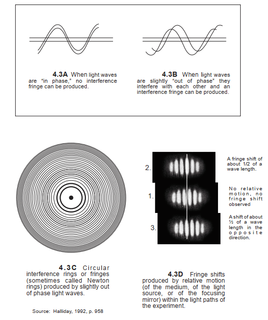
Another real, physical and empirical reason for Michelson’s so-called null results, which apparently has been completely overlooked by everyone, was that M & M were actually only attempting to measure (or compare) one slightly out-of-phase light wave relative to another slightly out-of-phase light wave (Picture 2). Such out-of-phase light waves created an interference fringe when Michelson slightly changed the distance of one mirror by fine tuning its micrometer screw. M & M then assumed that the solar orbital motion of the Earth would change the distance/time interval which one light wave would have to propagate away from the ether. But, to paraphrase Feynman, one can only assume that which one can measure, and one can only measure that which one can see. One cannot measure unobserved or undetectable phenomena.

Picture 2: Out Of Phase Light Waves Can Create An Interference Fringe, And Relative Motion Within The Light Paths Of The Experiment Can Create Fringe Shifts


Regardless of what M & M were assuming, and regardless of the direction that their apparatus might be pointing in, if the finite physical distance of each arm of his apparatus always remained the same, there could never physically be an interference fringe shift: that is, a change of the relative phase positions of such out-of-phase light waves. Stated somewhat differently: As long as the physical length of each arm did not change (whatever its magnitude of distance might be), the relative phase position of each out-of-phase light wave would physically have to remain the same. This was the empirical result of the 1932 Kennedy-Thorndike experiment where one arm was intentionally constructed much shorter in length than the other arm (Picture 3). Therefore, the specific finite length of each arm and the specific finite distance that each light ray propagated in any direction were always irrelevant to the occurrence of a fringe shift.

Picture 3: The 1932 Kennedy-Thorndike Experiment


For all of the above real, physical and empirical reasons, a fringe shift could never physically occur when Michelson or Kennedy pointed the arms of his apparatus in different directions over a period of several months. Michelson’s and Kennedy’s attempts to detect an interference fringe shift, or a difference in time intervals for light propagation in any direction, were always a mission impossible. In order to visualize what actually happened in Michelson’s experiments, refer to Picture 4.

Picture 4: Two Perpendicular Light Pencils Propagating Within Michelson’s Apparatus At 4 Different Times, In The Absence Of Stationary Ether


The next real reasons for Michelson’s null results are technical. We have already described one of these technical reasons. If the arms of Michelson’s and Kennedy’s experiments always remained the same finite length, then a fringe shift (a change in the relative phase position of two slightly out-of-phase light waves) never could have physically occurred (Pictures 3 and 5). The only way that a fringe shift could have occurred would be if Michelson or Kennedy would have slightly adjusted the distance of the focusing mirror with the micrometer screw in order to obtain a fringe (Picture 6). But since both scientists already had obtained an interference fringe, there was no reason for them to obtain another one. And they never did.

Picture 5: Michelson’s Interference of Light Experiments

Picture 6: What Happened When Michelson Adjusted The Distance Of One Mirror In The Path Of One Light Pencil?


A second technical reason was because M & M’s apparatus was located in the concrete basement of a building (with no windows) so that its sensitive instruments would not be affected by traffic, heat, sunlight, etc. If M & M had desired to visually detect the motion of the Earth’s solar orbital motion, or any other relative motion of the Earth, they could have mounted a 10-inch telescope on the roof of the building and observed the light paths of a passing luminous planet (i.e. Venus) or a luminous planet that the Earth was passing (i.e. Mars, Jupiter, or Saturn) through the lens of the telescope and calculated the solar orbital motion of the Earth over a period of months.

However, the solar orbital motion of the Earth could never be detected by the interference method employed by M & M or Kennedy & Thorndike from the basement of a building, because (unlike the telescope) there never was any material body which moved within the light paths of their interference experiment, which technically could be detected by any method. The only motion which occurred within the light paths of their experiments was when the focusing mirror was adjusted by the micrometer screw to create an interference fringe. For this simple technical reason, none of these scientists could ever detect anything else, and none of them ever did.


Source: The Michelson-Morley paradox solved (You can also read the whole treatise there)

The Experiment of Fizeau

The short description of the experiment of Fizeau:

1. When the water is not moving in each tube, the light propagating through each tube has the same velocity, so the light waves in the two pencils of light that reach the eye are in phase.

2. When light propagates through water moving in different directions at 7 m/s, the velocity of light relative to the tube increases in the direction of flow A and decreases in the opposite direction of flow B. Thus the light waves propagating through tube A will arrive at the eye sooner (and in less time) than the light waves propagating through tube B. This causes an out of phase interference of the crests and troughs of such light waves which is visible to the eye as a pattern of interference fringes. The distance between each dark fringe is one wave length.

Picture 1: The experiment of Fizeau which determined the velocity of light in a moving liquid

When the flow of the water in the tubes is reversed, the pattern of interference fringes shifts, and the measurable magnitude of this shift can be computed to determine the difference in the velocity of light propagating relative to each tube.

Maxwell’s 1879 Ether Assumptions

Picture 1: Light propagating in any direction on the theoretically stationary Earth


The Picture 1 also illustrates Michelson’s theoretical distance and time interval (T1) for light to propagate in the direction perpendicular to the Earth’s solar orbital motion.

Picture 2: Light propagating in the direction of Earth’s absolute solar orbital motion and away from the stationary ether


The Picture 2 also illustrates the theoretical in-tandem displacement of mirrors A and B with respect to the stationary ether. Because empirically there is no ether, these theoretical displacements from ether cannot occur.

The light source, the beam splitter (BS) and the mirror M are affixed to the surface of the Earth at a finite distance apart, and for purposes of illustration we assume that they move in tandem to the right at 50% of c relative to the stationary ether and the Sun theoretically at rest in the ether. A light ray leaves the terrestrial light source at some point A0 and transmits at 100% of c toward the mirror at some point M0. During such propagation, the mirror theoretically displaces from point M0 to some point M1 due to such absolute solar orbital velocity with respect to the stationary ether. The light ray contacts the mirror at point M1 after traveling (from A0 to M1). The light ray then reflects from the mirror at M1 and begins to propagate back toward the light source. During such propagation, the material light source theoretically displaces from point A0 to some point A1 and then to some point A2.
When the light ray returns to the light source at point A2 the light ray has traveled a total distance/time interval while the light source and the mirrors have theoretically displaced in-tandem 1/2 of the total distance, an increase of 1/4 of the total distance because of the theoretical displacement. These were also Einstein’s computations for a greater distance/time interval of light propagation, which he referred to in Relativity at pp. 58 - 59. On the other hand, if there had been no motion of the Earth in an absolute direction(and thus no absolute displacement), then the light ray would only have traveled a total distance/time interval of 3/4 of the total distance. Strangely enough is what actually happened, because there is no ether and there can be no physical displacement from something that does not exist.

Utilization of Radio Waves Energy

The method of utilization of the radio waves energy is kind of a derived idea from the Tesla's Method Of Utilizing Radiant Energy, as general concept. In this article, we analyze one simple electronic circuit which can be used as simple prototype for proving the concept of utilization of the energy of radio waves which propagates in the Earth's atmosphere all the time. These radio waves does not have a mysterious origin at all, as it can be found in many places on the internet sites which treats the so called "free energy" phenomenon. On the contrary, these radio waves are just real and known, human made signals. They origin from the base and repeater stations of the broadcasting network, comprising emitters of all local and national radio stations. The signal emitted from your favorite radio station which broadcasts program with music and news of your interest, is always present in the air around you, no matter if you catch that signal on your radio and listen its live program, or your radio is turned off. That signal is always there. And not just the signal from that particular radio station, which is your favorite, but also and all the other stations that emit their signals in your near or far environment.

So, if you chose not to listen the radio, that doesn't mean that you can not catch the radio signals around you, and try to utilize or store the energy that they carry out with them. Although this energy is relatively small, it can still be detected and accumulated on proper way, just as a proving fact that it exists in the air. Furthermore, since we know the origin of these radio waves, we can't say that the energy they carry around is "free", because we know that this energy is generated in the transmitter stations of the radio service which generated it. These radio transmitters doesn't work from nothing, they use electric power to generate the needed EM energy of the radio waves which they broadcast via the antennas, in their well known and pre-calculated range. Of course, the radio station is paying for the electric energy that it consumes, but the very small portion of the emitted EM energy that comes to your radio receiver via its receiver antenna at your home, you get it for free. However, this received energy is far different from the term "free energy" and its actual meaning.

The receiving circuit for utilizing radio waves energy

Let's now take a look at one real and simple circuit, which can accumulate the EM energy of radio waves via the receiving antenna. The utilization circuit is shown on Picture 1. The electrolytic capacitors C3 and C4 are used as elements for storing the energy, as they accumulate the charge from the incoming small-amplitude radio signals via the diode network which is constructed with 4 diodes D1, D2, D3 and D4, connected as shown in circuit (Picture 1). The capacity of the energy storing capacitors are set to relatively huge value of 1000 μF. The radio signals received from the antenna, are passed to the diode network via the signal block capacitors C1 and C2. Their value is set to 22 nF. Since we are simulating this circuit, we also need to simulate and the antenna as the most important circuit element here.

An antenna is best modeled as a voltage source with a fixed value of internal resistance. Generally, that is the radiation resistance of the antenna. So, in our circuit, we modeled the receiving antenna as a simple voltage source, with the series resistance value of 50 ohms. Although the voltage level of real radio waves is very small, we chose the value of magnitudes in this simulation which is far more higher, just for analyzing purposes. However, the concept of functioning of this circuit and its effect, will remain the same and for smaller and real values for the magnitudes of the incoming radio waves, except that the resulting values of the output voltage V+, will be much smaller, accordingly to the input signal values. But the important thing here, is to see that this idea as concept for utilization of the energy, really works. Therefore, for the antenna model used in our simulation, we use simple sinusoidal wave form, with magnitude of 200 mV at frequency of 500 kHz.

Picture 1: Utilization of Radio Waves Energy (simple circuit)

Time-domain analysis

The results of the transient analysis for this circuit in time domain are shown on Picture 2. For this analysis, the same simple sinusoidal wave form, with magnitude of 200 mV at frequency of 500 kHz, is used for antenna signal. As it can be seen from the plot, the output voltage level starts increasing with oscillating wave form, according to the input signal frequency. Starting from zero, the output level reaches value of about 14 μV after time period of 200 ms. The increasing rate is almost linear, so, after time period of 1 second, output will increase to value around 70 μV. This value is about 0.00035% of the input signal magnitude value. In other words, it's far more less than the input. So, in order to achieve really measurable voltage on the output of this circuit, the circuit should work for a long time, thus accumulating energy constantly. We have implemented one real prototype of this circuit, and the real results from practice showed us that the circuit should be left in accumulating mode for, let's say a period of one whole day, in order to achieve a value of several up to hundreds of mV on its output.

Picture 2: Transient analysis - output voltage V+ wave form (time-domain) - for single frequency input


The above results are in case of single-frequency input signal. As we now, in practice, the antenna will receive more than one signal, and all signals will have different frequencies. Furthermore, these signals are not simple and with pure sinusoidal form, since they are modulated in the proper modulation technique for radio transmission. So, the actual input signal received from the real antenna, would be a superposition of all radio signals that the antenna can receive in the environment where it is installed. However, for analysis purposes, we modeled another type of input antenna, which consists three different voltage sources connected in parallel, just to see the effect of the superposition of several signals at different frequencies. In our case, we set these three voltage sources with the following properties:

>> V1 voltage source: Frequency: 500 kHz; Amplitude: 200 mV; Wave form: sinusoidal;
>> V2 voltage source: Frequency: 100 kHz; Amplitude: 200 mV; Wave form: sinusoidal;
>> V3 voltage source: Frequency: 1 MHz; Amplitude: 200 mV; Wave form: sinusoidal;

Picture 3: Transient analysis - output voltage V+ wave form and input signal from Antenna (time-domain) - for 3 inputs at different frequencies

The resulting input signal wave form of the antenna is shown on Picture 3. On same plot is shown and the output voltage V+. As it can be seen, although all three input signals have same magnitude of 200 mV, because of their different frequencies, the resulting signal has amplitudes less then 200 mV. The final effect of this superposition is that the output voltage is increasing with slower rate, comparing with the previous case of one single-frequency input signal. So, after the time period of 200 ms, the output level will reach value smaller than 14 μV, as it reached in the previous case (Picture 2).

AC Analysis

The output voltage AC analysis of this circuit shows that it has higher output level as the frequency of the signal increase. For this AC analysis we set the frequency range of the input signal from 10 KHz to 10 GHz. Taking into account the whole Radio Spectrum which covers frequencies from 3 Hz up to 3000 GHz, this range that we analyze here is pretty much wide. The output voltage level at frequency of 10 KHz is -144 dB and it increases in linear mode up to frequencies of 100 MHz, where it reaches the level of -66 dB. After these frequencies, the output voltage is still increasing, but with slower rate. Finally, for frequencies above 1 GHz it stops to increase and its level remains at about -59 dB. The output level plot in frequency domain is shown on Picture 4.

Picture 4: AC analysis - output voltage V+ level (frequency-domain) - for single frequency input


Also, it's good to mention here, that in the lower frequency range of the radio spectrum, starting from 3 Hz to 10 KHz the output level is decreasing. Namely, at 3 Hz input signal, the output level is around - 100 dB, then it decreases with different speeds as frequency increases, so at frequency of around 3 kHz, it reaches the minimum level of around - 150 dB. For the frequencies above 3 kHz it starts to increase.

From the above analysis, we can conclude that this concept really works, but the amount of accumulated energy is not what we really expect and need in real applications. Since we talk about energy storing, we actually need amount of stored energy enough to power some small consumer, let's say LED diode light, or something else. In any case, this is just a simple approach of this concept. The circuit for utilization can be upgraded and optimized in many ways, in order to achieve better and usable effect in practice. The circuit can be split in several banks which will store energy from single-frequency signals, which should be previously demodulated and parsed by frequency, of course. Also, the receiving module can be implemented as antenna field, or system with more antennas, placed in some pre-calculated and optimized space constellation in that way that the received energy would be the maximum possible for the current system.

The real prototype of the circuit

 

Picture 5: The real prototype of the circuit for utilization of the radio waves energy


As we mention above, we have implemented one real prototype of this circuit, for testing and experiment purposes. The real prototype is shown on Picture 5. On this prototype circuit we have connected two antennas, removed from an old wi-fi repeater. The rest of the circuit elements are same as the circuit we simulated (Picture 1). Before connecting the antennas on the circuit, which is actually how this circuit is put in operation, we made sure that the energy storing electrolytic capacitors C3 and C4 are totally discharged. After putting the circuit in operation, next day the measured voltage of its output was 273 mV, as shown on Picture 6.

Picture 6: Measuring the output voltage of the real prototype (after 1 day of accumulation)

Maxwell's Equations

Maxwell’s Equations provide a general description of electromagnetic phenomena. They are named after James Clerk Maxwell, the Scottish physicist whose pioneering work unified the theories of electricity and magnetism. The theory of electromagnetism was built on the discoveries and advances of many scientists and engineers, but the pivotal contribution was that of Maxwell.

The properties of the microscopic electro-magnetic (EM) field for stationary environments are expressed with well known system of Maxwell's equations, as shown on Picture 1:

Picture 1: System of Maxwell's Equations (for stationary environments)


I. The first equation is derived in compliance of the Ampere's Law with the law of continuation.
II. The second equation is a generalized form of Faraday's Law for electromagnetic induction.
III. The third equation expresses the generalized form of the Gauss theorem.
IV. The fourth equation represents the Law of conservation of magnetic flux.


When solving concrete systems, the Maxwell's Equations system need to be upgraded or supplemented with the following equations (Picture 2):

Picture 2: Additional equations for general Maxwell's Equations System


Here, the equation (1) represents the generalized form of the Ohm's Law, while with the equations (2) are expressed the vectors of electric displacement and magnetic induction. For linear and isotropic environments, these equations (2), are expressed in the form as represented with the equations (3).

The physical quantities included in all these equations above, are:

E - Electric field;
H - Magnetic field;
D - Electric displacement;
B - Magnetic induction;
J - Electric current density;
ρ - Distribution of electric charge;
σ - Specific electric conductance;
P - Electric polarization vector;
M - Vector of magnetization;
ε - Electric constant;
μ - Magnetic constant;

Radio Communication

Propagation of Radio waves

Here we only look at the simple architecture of the radio system, a system for radio communication. The block diagram of the radio system is shown on Picture 1. As we can see from the picture, we have starting point for the signal (from its source) to the end of the radio link where this signal is received. So, the first part of the radio system is the source of signals (information). The source of signals can be anything, for example, a radio station. These primary signals are proceeded in the Radio-transmitter. Radio transmitter should process these signals in order to send them in the air (wireless) through its antenna. That means that transmitter should amplify the signal level (if needed), do the radio modulation of the signal - so the signal can be easily send in the air, and if there is need for protection of the information, it can also encrypt the signal with some pre-defined code, which is known only at the other side where this signal should be received.

After the signal is prepared for transmission, it travel through the air as EM (electro-magnetic) wave. Here we will not discuss about the propagation of the EM waves. The EM wave is exposed to disturbances in the point where it is generated (in the transmitter), all the way it travels (in the propagation environment) and in the point where it is received (in the receiver). The frequency carrier on which the modulated radio signal is transmitted is actually the transmission channel. The amount of disturbances and other critical parameters of transmission depends on the used frequency channel.

The radio receiver received the EM waves emitted from the the transmitter through its receiver antenna. This received signal is amplified, demodulated and decoded if it was previously coded, so it returns to its primary form as it was generated in the source, and finally it's send to the device for reproduction. So, on this way, the information is send through the air from point A (the transmitter) to point B (the receiver), and we can say that there is a radio communication between points A and B, which can be a miles away one from another, and the signals are send wireless (no need of cables) through the air.

Picture 1: Block diagram of radio system (propagation of radio waves)

Radio Spectrum

Radio spectrum is the part of the electromagnetic spectrum corresponding to the radio frequencies – frequencies lower than around 300 GHz.

The whole radio spectrum is divided into radio bands, and every band has name and purpose for use. There are 12 radio bands:


>> ITU radio band number 1: ELF - Extremely low frequency [3-30 Hz]; wavelength: 100,000 - 10,000 km;
>> ITU radio band number 2: SLF - Super Low Frequency [30-300 Hz]; wavelength: 10,000 - 1000 km;
>> ITU radio band number 3: ULF - Ultra Low Frequency [300-3000 Hz]; wavelength: 1000 - 100 km;
>> ITU radio band number 4: VLF - Very Low Frequency [3-30 kHz]; wavelength: 100 - 10 km;
>> ITU radio band number 5: LF - Low Frequency [30-300 kHz]; wavelength: 10 - 1 km;
>> ITU radio band number 6: MF - Medium Frequency [300-3000 kHz]; wavelength: 1000 - 100 m;
>> ITU radio band number 7: HF - High Frequency [3-30 MHz]; wavelength: 100 - 10 m;
>> ITU radio band number 8: VHF - Very High Frequency [30-300 MHz]; wavelength: 10 - 1 m;
>> ITU radio band number 9: UHF - Ultra High Frequency [300-3000 MHz]; wavelength: 1 m - 100 mm;
>> ITU radio band number 10: SHF - Super High Frequency [3-30 GHz]; wavelength: 100 - 10 mm;
>> ITU radio band number 11: EHF - Extremely High Frequency [30-300 GHz]; wavelength: 10 - 1 mm;
>> ITU radio band number 12: THF - Tremendously High Frequency [300-3000 GHz]; wavelength: 1 mm - 100 um;


According to the ITU Radio Regulations the radio spectrum shall be subdivided into nine frequency bands, those bands are from 4 to 12, or from VLF to THF. This spectrum is shown on the Picture 1.

Picture 1: The radio spectrum (ITU Radio Regulations)

Electromagnetic Spectrum

On Picture 1 is shown the electromagnetic (EM) spectrum. The wavelengths are represented in meters, the frequencies in hertzs. Also, on the picture is represented the energy of one photon for different frequencies of the EM waves in electron volts (eV). As we can see from the axis, the energy per photon increases as the frequency of the EM wave increases too (or the wavelength of the EM wave decreases).

The energy of one electron volt expressed in joule: 1 eV = 1.60217646 × 10^-19 J.

Picture 1: The Electromagnetic Spectrum (Source: Lawrence Berkeley National Laboratory)