Analog Inputs and Outputs

Many PLC-s also work with analog I/O devices. Analog devices use signals that are continuously variable within a specified range, such as 0 to 10 V DC or 4 to 20 mA. Analog signals are used to represent variable values, such as speed, rate of flow, temperature, weight, level, etc. In order to process an input of this type, a PLC must convert the analog signal to a digital value. Digital values from analog inputs are stored in addressable memory for use by the user program. Similarly, the user program can place digital values in addressable memory locations for conversion to analog values for the designated analog outputs.
Analog I/O points can be added using expansion modules for any CPU. The number of expansion modules depends on the CPU type and how many modules it can support. Expansion modules are available with 4 or 8 analog inputs, 2 or 4 analog outputs, or 4 analog inputs and 1 analog output (Or many other combinations, depending on the manufacturer and types). In addition, expansion modules are available for use with thermo-couples or RTD type sensors which sense the temperature at a specific point in a machine or process.

Analog Input Example

Analog inputs can be used for a variety of purposes. In the following example (Picture 1), a scale is connected to a load cell. A load cell is a device that generates an electrical output proportional to the force applied.

Picture 1: Analog Input Example


The load cell in this example converts a value of weight from 0 to 50 pounds into a 0 - 10 V DC analog value. The 0 - 10 V DC load cell signal is connected to an PLC’s analog input. The analog value applied to the PLC can be used in various ways. For instance, the actual weight can be compared to a desired weight for a package. Then, as the package is moved on a conveyor, the PLC can control a gate to direct packages of varying weight.

Analog Output Example

Analog outputs from a PLC are often supplied directly or through signal converters or transmitters to control valves, instruments, electronic drives or other control devices which respond to analog signals. For example, analog outputs from the PLC could be used to control the flow of fluid in a process by controlling AC drives (Picture 2). Rather than simply turning the AC drives on or off, which could be accomplished by discrete outputs, analog signals can be used to control the output of the AC drives. This would allow the speed of the pumps to be varied dynamically in response to changes in process requirements.

Picture 2: Analog Output Example

Discrete Inputs/Outputs

Motor Starter Example

A more practical, and only slightly more complex application is start-stop control of an AC motor. Before examining the PLC application, first consider a hardwired approach. The following line diagram (Picture 1) illustrates how a normally open and a normally closed push button might be connected to control a three-phase AC motor. In this example, a motor starter coil (M) is wired in series with a normally open, momentary Start push button, a normally closed, momentary Stop push button, and normally closed overload relay (OL) contacts.

Picture 1: Motor Starter Example


Momentarily pressing the Start push button completes the path for current flow and energizes the motor starter (M). This closes the associated M and Ma (auxiliary contact located in the motor starter) contacts. When the Start button is released, current continues to flow through the Stop button and the Ma contact, and the M coil remains energized.
The motor will run until the normally closed Stop button is pressed, unless the overload relay (OL) contacts open. When the Stop button is pressed, the path for current flow is interrupted, opening the associated M and Ma contacts, and the motor stops.

PLC Motor Control

This motor control application can also be accomplished with a PLC. In the following example (Picture 2), a normally open Start push button is wired to the first input (I0.0), a normally closed Stop push button is wired to the second input (I0.1), and normally closed overload relay contacts (part of the motor starter) are connected to the third input (I0.2). These inputs are used to control normally open contacts in a line of ladder logic programmed into the PLC.

Picture 2: PLC Motor Control


Initially, I0.1 status bit is a logic 1 because the normally closed (NC) Stop push button is closed. I0.2 status bit is a logic 1 because the normally closed (NC) overload relay (OL) contacts are closed. I0.0 status bit is a logic 0, however, because the normally open Start push button has not been pressed. Normally open output Q0.0 contact is also programmed on Network 1 as a sealing contact. With this simple network, energizing output coil Q0.0 is required to turn on the motor.

Program Operation

When the Start push button is pressed, the CPU receives a logic 1 from input I0.0. This causes the I0.0 contact to close. All three inputs are now a logic 1.
The CPU sends a logic 1 to output Q0.0. The motor starter is energized and the motor starts.
The output status bit for Q0.0 is now a 1. On the next scan, when normally open contact Q0.0 is solved, the contact will close and output Q0.0 will stay on even if the Start push button is released.
When the Stop push button is pressed, input I0.1 turns off, the I0.1 contact opens, output coil Q0.0 de-energizes, and the motor turns off.

Adding Run and Stop Light Indicators

The application can be easily expanded to include indicator lights for run and stop conditions. In this example (Picture 3), a RUN indicator light is connected to output Q0.1 and a STOP indicator light is connected to output Q0.2.
The ladder logic for this application includes normally open Q0.0 contact connected on Network 2 to output coil Q0.1 and normally closed Q0.0 contact connected on Network 3 to output coil Q0.2. When Q0.0 is off, the normally open Q0.0 contact on Network 2 is open and the RUN indicator off. At the same time, the normally closed Q0.0 contact is closed and the STOP indicator is on.

Picture 3: Run and Stop Indicator states


When the Start button is pressed, the PLC starts the motor. Output Q0.0 is now on. Normally open Q0.0 contact on Network 2 is now closed and the RUN indicator is on. At the same time, the normally closed Q0.0 contact on Network 3 is open and the STOP indicator light connected to output Q0.2 is off.

Further Expansion

The PLC program can be further expanded to accommodate a wide variety of commercial and industrial applications (Picture 4). Start/Stop push buttons, selector switches, indicator lights, and signaling columns can be added. Motor starters can be added for control of additional motors. Over-travel limit switches can be added along with proximity switches for sensing object position. Various types of relays can be added to expand the variety of devices being controlled. As needed, expansion modules can be added to further increase the I/O capability. The applications are only limited by the number of I/Os and amount of memory available for the PLC.

Picture 4: Expansion Elements

Basic Ladder Logic Symbols

PLC ladder logic consists of a commonly used set of symbols that represent instructions. Understanding these basic symbols is essential to understanding PLC operation.

Picture 1: NO/NC Contacts, Coil & Box

Contacts

One of the most confusing aspects of PLC programming for first-time users is the relationship between the device that controls a status bit and the programming function that uses a status bit. Two of the most common programming functions are the normally open (NO) contact and the normally closed (NC) contact (Picture 1). Symbolically, power flows through these contacts when they are closed. The normally open contact (NO) is closed when the input or output status bit controlling the contact is 1. The normally closed contact (NC) is closed when the input or output status bit controlling the contact is 0.

Coils

Coils represent relays that are energized when power flows to them (Picture 1). When a coil is energized, it causes a corresponding output to turn on by changing the state of the status bit controlling that output to 1. That same output status bit may be used to control normally open and normally closed contacts elsewhere in the program.

Boxes

Boxes represent various instructions or functions that are executed when power flows to the box (Picture 1). Typical box functions include timers, counters, and math operations.

Entering Elements

Control elements are entered in the ladder diagram by positioning the cursor and selecting the element from a list. In the following example shown on Picture 2 the cursor has been placed in the position to the right of I0.2. A coil was selected from a pulldown list and inserted in this position.

Picture 2: Entering Element in Ladder diagram

AND Operation

Each rung or network on a ladder represents a logic operation. The following programming example shown on Picture 3 demonstrates an AND operation. Two contact closures and one output coil are placed on network 1. They are assigned addresses I0.0, I0.1, and Q0.0. Note that in the statement list a new logic operation always begins with a load instruction (LD). In this example I0.0 (input 1) and (A in the statement list) I0.1 (input 2) must be true in order for output Q0.0 (output 1) to be true. This same logic is also shown in a function block diagram. The following truth table on Picture 3 represents the state of the output for each combination of input states.

Picture 3: AND Operation Ladder diagram

OR Operation

In this example (Picture 4), an OR operation is used in network 1. In the following example, if either input I0.2 (input 3) or (O in the statement list) input I0.3 (input 4), or both are true, then output Q0.1 (output 2) is true. The following truth table on Picture 4 represents the state of the output for each combination of input states.

Picture 4: OR Operation Ladder diagram

PLC Programming and Scan Process

Ladder Logic Programming

A program consists of instructions that accomplish specific tasks. The degree of complexity of a PLC program depends upon the complexity of the application, the number and type of input and output devices, and the types of instructions used. Ladder logic (LAD) is one programming language used with PLCs. Ladder logic incorporates programming functions that are graphically displayed to resemble symbols used in hard-wired control diagrams.
The left vertical line of a ladder logic diagram represents the power or energized conductor. The output coil instruction represents the neutral or return path of the circuit. The right vertical line, which represents the return path on a hard-wired control line diagram, is omitted. Ladder logic diagrams are read from left-to-right and top-to-bottom. Rungs are sometimes referred to as networks. A network may have several control elements, but only one output coil.

Picture 1: Ladder Logic Programming sample

Statement List and Function Block Diagrams

While ladder logic programs are still common, there are many other ways to program PLCs. Two other common examples are statement list and function block diagrams.
Statement list (STL) instructions include an operation and an operand. The operation to be performed is shown on the left. The operand, the item to be operated on, is shown on the right.
Function block diagrams (FBD) include rectangular functions with inputs shown on the left side of the rectangle and outputs shown on the right side.

In the following example (Picture 2), the program segments perform the same function.

Picture 2: STL, FBD, LAD samples


In addition to LAD, STL, and FBD, multiple other types of programming languages are used for PLCs. Each type of programming has its advantages and disadvantages. Factors such as application complexity, types of programming available for a specific PLC model, and user standards and preferences determine which type of programming is used for an application.

PLC Scan

The PLC program is executed as part of a repetitive process referred to as a scan. A PLC scan (Picture 3) starts with the CPU reading the status of inputs. Next, the application program is executed. Then, the CPU performs internal diagnostics and communication tasks. Finally, the CPU updates the status of outputs. This process repeats as long as the CPU in the run mode. The time required to complete a scan depends on the size of the program, the number of I/Os, and the amount of communication required.

Picture 3: PLC Scan Process

PLC-s

A programmable logic controller (PLC), also referred to as a programmable controller, is the name given to a type of computer commonly used in commercial and industrial control applications. PLC-s differ from office computers in the types of tasks that they perform and the hardware and software they require to perform these tasks. While the specific applications vary widely, all PLC-s monitor inputs and other variable values, make decisions based on a stored program, and control outputs to automate a process or machine.

Picture 1: PLC use

Basic PLC Operation

The basic elements of a PLC include input modules or points, a central processing unit (CPU), output modules or points, and a programming device (Picture 2). The type of input modules or points used by a PLC depends upon the types of input devices used. Some input modules or points respond to digital inputs, also called discrete inputs, which are either on or off. Other modules or inputs respond to analog signals. These analog signals represent machine or process conditions as a range of voltage or current values. The primary function of a PLC’s input circuitry is to convert the signals provided by these various switches and sensors into logic signals that can be used by the CPU.

Picture 2: Basic PLC Operation Elements


The CPU evaluates the status of inputs, outputs, and other variables as it executes a stored program. The CPU then sends signals to update the status of outputs. Output modules convert control signals from the CPU into digital or analog values that can be used to control various output devices.
The programming device is used to enter or change the PLC’s program or to monitor or change stored values. Once entered, the program and associated variables are stored in the CPU. In addition to these basic elements, a PLC system may also incorporate an operator interface device to simplify monitoring of the machine or process.

In the simple example shown below (Picture 3), push buttons (sensors) connected to PLC inputs are used to start and stop a motor connected to a PLC output through a motor starter (actuator). No programming device or operator interface are shown in this simple example.

Picture 3: Example - PLC in use of starting of motor

Hard-wired Control

Prior to PLC-s, many control tasks were performed by contactors, control relays, and other electro-mechanical devices. This is often referred to as hard-wired control. Circuit diagrams had to be designed, electrical components specified and installed, and wiring lists created (Picture 4). Electricians would then wire the components necessary to perform a specific task. If an error was made, the wires had to be reconnected correctly. A change in function or system expansion required extensive component changes and rewiring.

Picture 4: Hard-wired Control Circuit

Advantages of PLC-s

PLC-s not only are capable of performing the same tasks as hard-wired control, but are also capable of many more complex applications. In addition, the PLC program and electronic communication lines replace much of the interconnecting wires required by hard-wired control. Therefore, hard-wiring, though still required to connect field devices, is less intensive. This also makes correcting errors and modifying the application easier.

Some of the additional advantages of PLC-s are as follows:

• Smaller physical size than hard-wire solutions;
• Easier and faster to make changes;
• PLCs have integrated diagnostics and override functions;
• Diagnostics are centrally available;
• Applications can be immediately documented;
• Applications can be duplicated faster and less expensively.

Fault Finding and Analysis

Fault finding

Picture 1: Acquisition of actual status


The actual fault finding starts once the actual status has been established and compared with the required status. This comparison frequently leads to the discovery of the error source, if the fault is:

>> visible (e.g. mechanical damage to a signal generator);
>> audible (e.g. leakage on a valve);
>> detectable by smell (e.g. cable burnt out).

If this is not the case, the fault can only be found and eliminated by means of a systematic procedure.

Systematic fault finding

Again, the required/actual status comparison forms the basis for systematic fault finding (Picture 2).

Picture 2: Systematic fault finding

Fault documentation

Once a fault has been found, it is not sufficient just to rectify this, but at the same time the cause of the problem should be determined. A useful tool for this is a faults list, which should be kept with the installation. This list describes the malfunctions and their causes. It may take a number of different forms.

The following is an example (Picture 3).

Picture 3: Fault documentation table - example

This list can be useful in detecting frequently recurring faults and their causes. The fault index makes it easier to establish the nature of the error:

A = Incorrect working practice (e.g. a retaining screw is not properly tightened on an assembly part);
M = Mechanical fault (e.g. sensors are maladjusted);
E = Electrical fault (e.g. relay is not energised or solenoid does not switch);
S = Controller error (e.g. program or program part is not activated);
L = Leakage fault (e.g. water escaping from threaded connection);
B = Operator error (e.g. shut-off valve not closed);
W = Service error (e.g. filter not cleaned).

Fault analysis

With the help of the faults list, it is possible to establish whether a fault or damage occurred and thus to pinpoint weak points in the system. Once these have been identified, it is advisable to introduce technical improvements. If damage has occurred, the following procedure should be adopted (Picture 4):

Picture 4: Fault analysis procedure

Final analysis

Fault finding and elimination means not just to render the system operational again, but also to identify and improve weak areas in the system.
The basic prerequisite for this is a knowledge of all control technology aspects and understanding of the function and interaction of hybrid systems.

Systematic Repairs in the Event of Malfunction

In the event of an inadvertent interruption, repairs are to be carried out according to the following plan (Picture 1):

Picture 1: Systematic repairs

Prerequisite for systematic repairs

The basic prerequisite for systematic repairs and fault finding is knowledge of the system. This means that only when you have familiarised yourself with the system and know how it is structured, will you be able to carry out systematic repairs. Familiarisation with the system by:

>> closely observing the installation;
>> making available the entire system documentation;
>> knowing the product and processing technology;
>> exchanging information with the user, operator.


Structuring of the system into:

1. System and controller structure

>> Program flow charts
>> Function charts
>> Description

2. Mechanical design

>> Structure and support unit
>> Function units
>> Adjustment

3. Drive technology

>> Electrical system
>> Hydraulics
>> Pneumatics
>> Mechanical system

4. Final control element

>> same as 3

5. Control system

>> Electrical relay control
>> Programmable logic controller

6. Signal generator

>> Binary sensors
>> Analogue sensors
>> Digital sensors

7. Power supply

>> Electrical
>> Hydraulic
>> Pneumatic

Procedure

The first thing that must be done in the event of an error signal is to establish the actual status. The following options are available for this:

>> Discussing the fault with the user (Does the system operate incorrectly?);
>> Start failure;
>> Stopping during process step;
>> Faulty process;
>> Incorrect working practice.

Maintenance

The term maintenance refers to all measures regarding the preservation and re-establishing of the setpoint status and the determining and evaluation of the actual state of technical resources of the system (DIN 31051). More specifically, maintenance can be divided into three areas (see Picture 1):

>> Service;
>> Inspection;
>> Repairs.

Picture 1: Areas of maintenance

Service

The term Service refers to preventive measures to prolong operating times. Servicing of technical installations covers (Picture 2):

Picture 2: Service

Inspection

Picture 3: Inspection

Repairs

 

Picture 4: Repairs

Fault Finding and Error Handling

Damage prevention training

Fault finding and error handling represents an extensive area of functions in a an operational technical process. A wide variety of errors can occur, which need to be analysed and eliminated by maintenance personnel. As far as a systematic grouping of these errors is concerned, Picture 1 defines different categories which are discussed below.

Picture 1: Classification of malfunctions in automation systems


Group 1 covers the typical errors, which are caused as a result of a failure of sensors or also non-operational actuators. Here, the following advice is given for error elimination:

Category 1

Sensor faults

>> Metrological checking immediately at the sensor terminals themselves or on the EMCS field terminal points.

Actuator faults

>> Testing of the incoming control signal on the actuator;
>> Testing directly on the actuator – signal path from the positioning to the servo drive (checking of calibrating accuracy);
>> Testing directly on the actuator – mobility of the valve poppet and spindle (error – e. g. as a result of jamming or rusting of valve poppet or spindle).

Category 2

Errors in transmission lines

>> Transmission measurements by means of checking of terminals on the EMCS field terminal points and process control console;
>> Visual checking of cable guides or cable trays (cable racks) to determine any mechanical damage.

Category 3

Errors in transmitter technology

>> Checking of input/output behaviour by applying defined input signals to the input terminals of the measuring transducer;
>> Checking of or repeating the calibration of the measuring transducer (checking of supply voltage).

Category 4

Errors on processors

>> Checking of supply voltages;
>> Checking of input/output signals according to allocations resulting from algorithm processing (e. g. off-line testing of PLC or compact controller).


Apart from the above mentioned typical errors on technical process systems, which can generally always be eliminated with the help of appropriate know-how, malfunctions can also occur, which may lead to damage of entire system complexes, including personal injury or at the very least serious danger. However, with the help of so-called damage prevention training, all system personnel are trained in how to react sensibly in the event, particularly of disaster, and to minimise any unavoidable material or personal damage. Doubtless, this damage prevention training is of particular importance in high risk installations (e. g. in atomic power stations, power stations, chemical plants, etc., but generally always needs to be adapted to the actual process technology.


A number of fundamental main points are listed below regarding the essence of damage prevention training:

>> First of all, the technical process system is to be broken down into important individual sections from the point of view of process technology and system safety.
>> Personnel are then to be completely familiarised with this structural breakdown (individual sections and their interaction), e.g. small-scale experimental module divided into the individual sections of filling level, flow and temperature control systems and supply module).
>> On the basis of the breakdown of the system structure, a strategy is to be developed for the isolation of individual technical process system sections. To this end, manual intervention (emergency intervention) with the help of the designed automation systems should be possible which, owing to the configuration of the transmission lines (e. g. stainless steel pneumatic lines), ensures a refractability of at least 1 to 2 minutes even in an emergency.
>> Personnel are to be trained in the handling of these emergency interventions.
>> Furthermore, appropriate fire extinguishing and other damage controlling devices are to be incorporated in the emergency operation training.
>> Finally, the most effective withdrawal of personnel from a damaged installation is to be defined and taught in the event of any damage occurring.
>> Personnel must also be given training in recognising any damage which has occurred as a result of an emergency (e. g. environmental damage), plus any other systems including personnel in danger, and in informing any other parties in close proximity as appropriate (to be evacuated) or to include these in the damage control.

Upkeep of Technical Process Systems

(small-scale experimental module)

Undoubtedly, the extent and cost of maintenance of modern technical process systems is to a large extent determined by the quality of the automation system (the automation project), whereby the use of modern automation equipment plays a vital role. Here, it should be acknowledged that the recognised procedure for conventional instrumentation has to be reconsidered for the maintenance and commissioning of a technical process system. In this context, the following aspects should be taken into account:

>> Modern automation equipment is highly reliable, requires little or no readjustment, or can be easily adjusted via control and instrumentation systems or similar control elements, whereby any readjustments can be easily made if required.

>> The universal use of process control engineering, being a typical characteristic of modern automation systems, facilitates a new and efficient approach to realising the required measures for maintenance and upkeep.

>> The emerging use of fieldbus systems (bus systems in effect) similarly is to be taken into consideration and also influences the maintenance and upkeep operations.

It is therefore essential, in particular as far as advanced process technology systems is concerned, to reconfigure any previously used maintenance and upkeep strategies, whereby the tried and tested (from previous practice) should be adopted and new strategies (e.g. by evaluating the above points) should at the same time be pursued.

Establishing the Standby Mode of a Technical Process

By utilising the available auxiliary energy (electrical and pneumatic) and the operational automation configuration (binary control systems and closed control loops in manual mode), the technical process is to be put into standby mode, which guarantees the activation of the actual steady-state operation of the continual process. In particular, the following preparatory steps are to be carried out:

>> Filling and venting of necessary piping sections to ensure the delivery capacity of the pumps used.

>> Provision (pump supply) of a sufficient quantity of materials to the output containers.

>> Configurational changes to container and piping system for the production start-up by means of actuation of selected on/off valves and corresponding hand valves.

Testing of Closed Control Loops, Binary Control Systems and Safety Devices

When the required auxiliary energies have been made available, the testing of the automation configuration/structure can be started. The following procedure is recommended to successfully realise this task (Picture 1).

Picture 1: Testing of automation configuration of a technical process system


With step 1, the binary control systems are tested as a first measure. This involves, for example, the testing of the on/off valves provided for configurational changes and their interaction with the corresponding binary controllers. In this connection, the signals resulting from the so-called final control element feedback in particular are to be evaluated visually or by means of binary monitoring (binary control systems). Similarly, the allocated binary control systems for the switching on and off of corresponding pumps and heaters are to be tested. Here again, the allocated binary control systems are to be tested via the manual control elements and corresponding feedback sensors.

Equally, the testing of safety devices also includes the monitoring of binary control systems. However, to do this, the associated sensors are to be activated by means of suitable manipulation and any actuators thus actuated evaluated in the familiar manner for correct functioning (visual and logic final control element acknowledgement). If the binary control systems including safety devices are then fully functional, the actual commissioning of the closed control loop can be started. To do this, the closed control loops are brought into line with the respective specified working points in manual mode and then switched over to automatic mode. After a sufficiently long evaluation of the guiding and interference behaviour of the activated closed control loops, the system can be handed over to the user.

Connection of Auxiliary Energies

The main concentration of work concerning the connection of auxiliary energies (electrics, pneumatics, hydraulics) is on the electrical auxiliary energy. This form of auxiliary energy is the dominant factor in the operation of an automation system.

Picture 1: Principal aspects regarding the connection of electrical auxiliary energy


Because of the different groups of consuming devices, the sequence of connecting different voltage levels is determined and a procedure (steps 1 to 3) introduced as shown in Picture 1, whereby these voltages are made available:

Step 1:

Connection of electrical auxiliary energy for processors (process control system, compact controller, PLC technology and PC’s):

>> Typical voltage levels:
- 230 V AC;
- 24 V DC (made available via power supply units).

Step 2:

Connection of electrical auxiliary energy for automation equipment – standard consuming devices (such as sensors, actuators, measuring transducers and safety devices):

>> Typical voltage levels:
- 230 V AC (main supply);
- 24 V DC (made available via power supply units).

Step 3:

Connection of electrical auxiliary energy for automation equipment – Large consuming devices (such as pumps and heaters):

>> Typical voltage levels:
- 400 V AC (main supply);
- 230 V AC.


Picture 2 to Picture 5 provide examples of this, which represent technically, a typical circuit solution in line with the connection procedure (steps 1 to 3). Picture 2 shows an example of how, by implementing steps 1 to 3, the electrical auxiliary energy for the small-scale experimental module is to be connected. This illustrates that the compact controller (processor) is the first to be supplied with auxiliary energy, followed by the sensors, actuators, small pumps and safety devices and, finally, the heater (being a large consuming) device.

Picture 2: Connection of electrical auxiliary energy using the example of a small-scale experimental module


An individual example then illustrates, which proposed circuit is more favourable for the supply of electrical auxiliary energy for the processors (Picture 3), whereby the safety device as well as the pneumatic auxiliary energy is supplied via the additional contacts of contactors K1 and K2. (Picture 5). Picture 4 demonstrates an example of the connection of electrical auxiliary energy for large consuming devices, whereby the allocated pumps and heaters are supplied with the required 40 V AC via contactors K3 to K6.

Picture 3: Connection of auxiliary energy for processors

Picture 4: Connection of electrical auxiliary energy for heavy consuming devices

Picture 5: Connection of pneumatic auxiliary energy

Commissioning of Process and Automation Systems

Commissioning strategy

To be able to solve the tasks set out in the main heading, it is first of all necessary to establish that the process technology system (the process) and the automation system should always be regarded as one entity. In this respect, the interaction between process (process technological system section) and the automation structure should always be taken into account as far as commissioning is concerned. Picture 1 therefore provides an overview of the main aspects of commissioning of process and automation systems, categorised into levels I and II. Here, it is of major importance, in which order (according to which commissioning strategy) the individual commissioning actions are carried out, thus determining the actual time period, costs arising and the success of system commissioning.

Picture 1: Main activities involved in the commissioning of technical process systems


A first evaluation of Picture 1 enables you to define the following main activities for commissioning:

Level I

Group 1 (step 1)

>> Connection of electrical (and pneumatic) auxiliary energy for processors and other automation equipment (with the exception of large electrical consuming devices).

>> Checking the operating mode – manual mode – for the existing closed control loops and binary control systems on the technical process system.

>> Basic test of binary control systems, e. g. for the switching on and off of pumps, open/closed valves, etc., structure variations of the system and the testing of monitoring equipment.

Group 2 (step 2)

>> Establishing the operational readiness of the process, e. g. availability of required media (basic materials) in the appropriate output containers, necessary filling of piping systems, etc., (all operating steps in manual operation).

Group 3 (step 3)

>> Testing of safety devices (as specified in VDI/VDE 2180), whereby safety device 1 (sensors, actuators and processor algorithms are to be tested first, followed by safety device 2.

>> Connection of electrical auxiliary energy for large consuming devices.

>> Approaching of the working points of the process technological system, i.e. the closed control loops are moved into the required working points in manual mode, whereby the controller structure and the controller parameters are programmed for each closed control loop.

Level II

Group 1

>> Establishing of operating mode – automatic mode – by means of a smooth transition, manual/automatic changeover (control signal-manual and control signal-automatic coincide).

>> Monitoring of steady-state initial start-up and testing of control and disturbance behaviour.

Process Protection Measures

Since the previous articles solely represented an account of the main aspects of project design work, the question of process protection has not been dealt with explicitly. It therefore has to be said that this question can be a particularly important additional factor of project design work in relation to process technology. For example, the requirements for the automation of an atomic power station will be considerably higher than those for the automation system of a brewery. Consequently, the project design engineer must be aware of the respective essential requirements for process protection and incorporate these into the project design. Picture 1 sets out the basic aspects of process protection.

Picture 1: Overview of basic aspects of process protection


According to this, the project design engineer will be confronted with problems such as explosion protection (explosion-proof design of automation equipment and systems). There is generally sufficient company documentation available for this, whereby the requirements arising from process technology can be implemented quite successfully.

The problem of EMC (electro-magnetic compatibility), which is also shown on Picture 1 is even more complex compared to an explosion proof design of automation equipment. However, depending on process requirements it also needs to be taken into consideration in the design of an automation system. Here, the project engineer’s experience is of some importance, since the appropriate know-how is at best only partially available in technical literature. It is therefore, as previously mentioned, up to the experience of individual companies to realise a well configured automation, system as far as EMC is concerned.
Similarly, the problem of lightning protection must be accorded its proper place in this context, since it also plays an important role in advanced system automation. Again, only fragmented specifications can only be found in the technical literature, including DIN documentation, hence the experience of the project design engineers is again crucial as far as this aspect of process protection is concerned. Apart from the above mentioned topics, which doubtless require further details, there remains the important matter of VDI/VDE2180. This guideline is of the greatest practical relevance and is to be incorporated unequivocally and practically in the project design.

Picture 2: Mode of operation of monitoring and safety equipment


VDI/VDE guideline 2180 is based on the following basic precept. (Picture 2):

>> Case 1: In the case of a process technological system, differentiation is made between the so-called acceptable range, the permissible error range and the unacceptable error range. Here, it is assumed that a process technological system in the course of normal operation (steady-state operation) moves within the so-called acceptable range, i.e. in the event of a drifting of process parameters from the working point, the system operates in the permissible error range. The protection of this operating regime is realised by means of the actual automation system, whereby a corresponding monitoring device (limit value encoded) ensures that if the acceptable range is exceeded (steady-state operating status), the system is automatically returned to the acceptable range or, if governed by the process technology, by manual intervention.

>> Case 2: If this monitoring device fails, then a so-called safety device (safety device 1) is indicated, which is also realised by means of a corresponding limit value encoder and at the very least returns the process parameters into the permissible error range.

>> Case 3: Irrespective of these measures described, an additional safety device (safety device 2) must be provided, which comes into effect in the event of failure of the previously described safety technology. This safety device requires a hardware basis which is completely independent of the previous automation equipment, which encompasses both sensors and actuators and also processors.


This ensures that in the event of failure of monitoring or safety equipment 1, an additional automation structure becomes effective in the process technology system, thereby preventing any drifting of the process parameters into the unacceptable error range (system damage or breakdown). Depending on the process class, the project design engineer must therefore decide to what extent the specifications of VDI/VDE 2180 must be incorporated in the project design work.

Selection of equipment - The Final Control Element

Selection of the final control element (regulating valve / control valve / valve actuator)

The function of a final control element in a piping system is to change the fluid throughput by means of its variable flow resistance. Picture 1 provides a schematic representation of customary final control elements, of which the control valve is undoubtedly the most frequently used regulating device.

Picture 1: Final control elements in flow technology


Picture 2 therefore illustrates the design of a control valve (schematic), whereby an equivalent electrical circuit diagram is also provided to facilitate any possible similar considerations (Picture 3).

Picture 2: Design of a control valve


Faced with the task of selecting a final control element, the first step is to examine the basic behaviour of the final control element in a system section (pipe section). In this context, it should be noted that due to the flow resistance of this final control element, a dynamic pressure drop occurs ∆p, which quadratically depends on the flow velocity or throughput. This means that part of the overall pressure available at the start of the pipe is reduced in the final control element (loss of energy).

Picture 3: Equivalent electrical circuit diagram of a control valve


Due to its nature, it follows that a process technological system will always be equipped with numerous control valves, in that different flow and pressure conditions will occur. It is therefore necessary to introduce the main parameters and facts in order to classify these control valves. To be able to make a permanently (experimentally) reproducible comparison of control valves, manufacturers work on the basis of a standard state (standard flow rate) of the valve to be used and define the so-called kv value. This means that for a pressure drop of 0.98 bar (0.98 − 105Pa), manufacturers specify water flow rates of (ρ = 103 kg/m3) passing through the valve. These standard flow rates depend purely on the valve stroke y and are referred to as kv value. The throughput associated with the nominal stroke of the control valve is known as kvs value.

The dependency of the kv values on the respective valve stroke is recorded in the so-called steady-state characteristic curve or basic characteristic curve of the control valve. The most typical basic forms of this basic characteristic curve can be most frequently found in:

>> the linear characteristic curve (a variation of valve stroke causes a change in linear throughput – see Picture 4);
>> the equal-percentage characteristic curve (variation of valve stroke and throughput have a non-linear correlation – see Picture 4).

Picture 4: Basic characteristic curve of control valves


On the basis of the actual automation task (design of process technological system section) it has to be decided, which basic characteristic curve is to be used. To give a practical indication, the following procedure can be recommended:

If the static characteristic curve is known (estimation) for the process technological section intended for the use of the valve, then the basic characteristic curve of the control valve is to be selected in such a way that, with the added superimposing of both characteristic curves (with the interaction of system section, and control valve) a as near as possible linear steady state characteristic curve (operating characteristics) is obtained for the flow behaviour.

Furthermore, it should be noted that various control valves, depending on the constructional design, do not completely seal during a zero valve stroke. The resulting residual throughput is referred as the kVo value of the control valve. From the point of view of cost and function, this should not necessarily be regarded as a disadvantage, since the comparatively simple On/Off valves are often used to completely close off pipes. Moreover, the control valve can be fashioned into a completely closing version by means of corresponding design changes (e. g. use of compressible seals). In this case, one also speaks of the so-called zero-point suppression. In this case, the characteristic curve greatly deviates from the actual basic characteristic curve in the case of a small stroke (Picture 5).

Picture 5: Linear basic characteristic curves of control valves with and without zero suppression


The parameters kvs and kvo are used to form the so-called theoretical control ratio kvs/kvo, which is generally specified as a typical parameter by the valve manufacturer and, in practice is often also replaced by the effective control ratio kvs/kvr. This takes into account the tolerance between the targeted and the actually measured basic characteristic curve (see also Picture 5).

If we now turn to the impending valve selection then, according to the above information, we start with the kv value. For a pressure drop ∆p≈1bar (specification resulting from practical experience) this can be determined as follows by the project engineer, taking into account the flow rate of the system section (specification resulting from practical experience:

Kv = 0.032 * q * √(ρ/∆p)

q – Output flow in m3/h (flow rate);
ρ – Density of passing medium in 103kg/m3;
∆p – Pressure drop via control valve (specification 1 bar).


This means that by defining (estimating) the maximum and minimum flow rates (qmax/qmin) in the system section in question, the following characteristic values are calculated with the help of the above formula:

kvs = 0.032 * qmax * √(ρ/∆p)

(maximum valve stroke y/ also Kv max) and

Kvmin = 0.032 * qmin * √(ρ/∆p)

(minimum valve stroke y).

For practical purposes, it should be noted that, in most cases it is not possible to find a control valve with the kvs value calculated from the system data. Consequently, for practical reasons, (e. g. also taking into account any other occurring changes in the system data) one should always select a control valve with a higher kvs value (than that calculated), i.e. the control ratio kvs/kvr.

Additionally, it should be mentioned that by changing the formula to determine the kv value, it is also possible to obtain a formula for the above mentioned operating characteristics, which is as follows:

q = kv * 31.62 * √(∆p/ρ) = g (y, ∆p)


However, in this case ∆p represents the actual pressure drop via the control valve for the respective flow rate, which can only be recorded metrologically, but in practice is not realised in the form of a measuring point. The formula is therefore less relevant in practical terms and the satisfactory (practically linear) operating characteristic can only be achieved by means of the already mentioned superimposition of basic characteristic curve and system characteristic curve. In conclusion, a few comments should also be added with regard to the classification /estimation of the steady-state characteristic curves of process technology system groups. As can be seen from Picture 8, differentiation is made between system sections with dominant static pressure drop and dominant dynamic pressure drop. However, in Picture 6, it can be clearly seen that in systems with static pressure drop, this only marginally depends on the flow rate, also known as output flow q.

Picture 6: System with steady-state pressure drop (ideal case – pump resistance neglected)


It therefore generally applies that the overall pressure drop remains constant and as such also the pressure drops via the system section and control valve. In the case of system sections with dynamic pressure drop, the pressure changes in relation to the output flow q and via the system section itself, and via the control valve as per Picture 7.

Picture 7: System section with dynamic pressure drop (ideal case – pump resistance neglected)


Picture 8 represents a summary of the main considerations involved in selecting a control valve, which are documented in the form of basic rules of procedure via points 1 to 4.

Picture 8: Selection of a control valve

Selection of sensors

As a rule, the selection of sensors within the framework of an automation project is more straightforward than the selection of actuators described in the last section. The selection by means of evaluating the respective company literature is relatively simple for the project engineer. By using the measuring ranges associated with process technology, all that remains for him to do is to select a corresponding sensor. Picture 9 illustrates this procedure. Needless to say, the environmental operating conditions of the sensor also are to be taken into account (e. g. aggressive medium, assembly conditions, etc.).

Picture 9: Selection of sensors

Selection of equipment - The Centrifugal Pump

Using the example of flow and filling level control you are familiar with from the small-scale experimental modules, there now follows an explanation of the essential fundamentals of the theory of flow. Both closed control loops start from the premise of one fluid flow (water throughput), whereby flow q and pressure p represent the characteristic process parameters. Here, it should be noted that in the relevant literature on pump function and pump design, the term ’output flow’ is often used instead of flow rate.

The object of the exercise now is to realise a corresponding flow rate or output flow for the respective specifications. In process technology, centrifugal pumps (also adjustable) and control valves are primarily used for this purpose. Picture 1 initially provides a more detailed account of the design and configuration of the centrifugal pump.

Picture 1: Design of a centrifugal pump (front and side view)


The most important characteristic of the centrifugal pump is the unclosed pump chamber, whereby the fluid is sucked into the pump housing, accelerated by the rotating impeller and due to the available centrifugal force forced through the outlet opening again. This creates a pressure difference between the pump inlet and outlet, whereby a vacuum is created on the pump input side as a result of the outward flow of the fluid from the impeller axis. Consequently, if for instance the pump draws in fluid from a container at a lower level, the lift is limited by the difference between the container vacuum and achievable vacuum.
If a vacuum is created on the pump input side, which is less than the so-called vapour pressure of the fluid, this results in evaporation, so that when the created gas bubbles are imploded this may lead to damage of the impeller in areas of higher pressure. This phenomenon is known as cavitation.
Moreover, the constructional design of a centrifugal pump means, that it cannot be closed off. With excessive reverse pressure, this leads to an opposing flow. To prevent this, a non-return valve is to be fitted in the pipe downstream of the pump, which only opens if there is a delivery pressure.
However, a centrifugal pump is also able to operate for a shorter period of time against a closed valve (shut-off valve) without overloading or damaging the drive unit. In the case of large centrifugal pumps, it is necessary to keep the shut-off valve closed during start-up and shut-down.
Furthermore, the centrifugal pump is characterised by the so-called Pump characteristic curve. This indicates the correlation between output flow and delivery pressure at a constant speed. With increasing output flow, a rising pressure drop is created on the internal flow resistance of the pump housing and guide blade. In an ideal case, the delivery pressure of the pump will be ∆p, whereby applies:

∆p = ∆p0 − ki * q^2

∆p – Delivery pressure;
∆p0 – Maximum delivery pressure (at Q=0);
ki – Fluidic constant of pump;
q – Output flow.

As an addition, Picture 2 illustrates the equivalent electrical circuit diagram of a centrifugal pump and should be regarded in this sense as a reference to possible similar considerations, which will however not be dealt with in this context.

Picture 2: Equivalent electrical circuit diagram of a centrifugal pump


ps – Pressure on pump suction side/vacuum;
pD – Pressure on pump delivery side/excess pressure;
∆pi – Pressure drop subject to internal resistence of pump;
∆p = ∆po - ∆pi - corresponds to differential pressure between pump output and input side.


Very often the delivery pressure ∆p, the delivery head h in relation to a specific fluid, is often specified as a typical pump parameter as an alternative to delivery pressure, e. g. example for water (density p = 1 g/cm3), the delivery head is calculated as:

h = ∆p/(ρ * g)

This is how corresponding characteristic curves are obtained for different speeds (Picture 3) and the fundamentals of the efficiency factor of a centrifugal pump can be discussed.

Picture 3: Qualitative representation of pump and efficiency characteristic curves


With an output flow of zero (point A in Picture 3), i.e. the pump is operated against a closed valve or the static differential pressure in a pipeline is identical to the delivery pressure, this results in a situation where, although the pump is working, no fluid is transported. This means that efficiency is 0 and the energy consumed is converted into heat in the pump housing. However, over an extended period and with insufficient cooling, this may lead to pump damage, whereby this working point can no longer be maintained over an extended period.
Once the output flow has increased, the pump reaches its maximum efficiency (point B) at a working point. If the output flow further increases (point C), the recorded drive capacity increases, which leads to a deterioration in efficiency in the case of a squared degressive delivery pressure. The increase in power consumption may lead to overloading of the drive motor. This is why a predetermined output flow must not be exceeded. If you now assume the task of selecting a centrifugal pump, this process of selection can be conducted along the lines of a relatively simple procedure.
First of all, differentation must be made between two types of pump application. In the first case, the pump is used as a pressure increase facility to maintain the flow (of the output flow) in a pipe, whereby the pump operates at a constant speed. In the second case, the pump is used as a throughput regulating element, whereby its speed is used as a correcting variable.

Picture 4 deals with the first case, i.e. the pump operates at a constant speed. In addition, the steady-state characteristic curve of the pump and system (system section) are entered in a diagram (Picture 4) and the planned working point of the pump defined at the point of intersection of the pump characteristic curve and system curve. Furthermore, the efficiency of the pump is also used to determine the working point (the nominal ratios) (Picture 5).

Picture 4: Selection of a centrifugal pump with the help of the steady-state characteristic curve of system section and pump (qo – delivery rate within working point)

Picture 5: Efficiency of centrifugal pump in relation to delivery rate (q0 – delivery rate within working point)


This means that apart from defining the working point of the centrifugal pump (output flow q0) at the intersection of the above characteristic curves, it is also necessary to take into account the maximum efficiency as a specification for the output flow q0. Depending on the pump selection available, it is often not possible to avoid a compromise in the sense of deviations from ηmax.
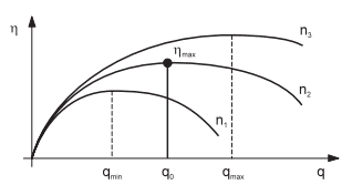
In the case of the centrifugal pump with variable speed, the basic requirement – definition of qmin and qmax – must be met to begin with (in accordance with corresponding process technological specifications) (Picture 6).

Picture 6: Characteristics of a pump with variable speed range (q0 – Delivery rate within working point)


Furthermore, the speed range /control range (speeds n1 to n3) of the pump to be selected are to be defined. To this end, the characteristic curves shown in Picture 6 illustrate, that any volumetric delivery can be achieved by varying the speeds of the centrifugal pump. As far as the optimum pump selection is concerned, one should again aim for a pump speed to be effective in the working point (output flow q0), which also represents the best possible efficiency for the output flow q0. The required efficiency ηmax in this case is also available in the form of a characteristics field (Picture 7) whereby, as already explained, a compromise to a certain extent is unavoidable, since the intersection of the pump characteristic curve (speed at working point – e. g. n2) and system characteristic curve do not always ensure the most optimum efficiency ηmax (see Picture 7).

Picture 7: Efficiency characteristics of a centrifugal pump in relation to the delivery rate (q0 – Delivery rate within working point)


Based on a summary of the above mentioned descriptions, the following schematic drawing on Picture 8 is obtained for the pump selection.

Picture 8: Selection of a centrifugal pump