Selection of the final control element (regulating valve / control valve / valve actuator)
The function of a final control element in a piping system is to change the fluid throughput by means of its variable flow resistance. Picture 1 provides a schematic representation of customary final control elements, of which the control valve is undoubtedly the most frequently used regulating device.
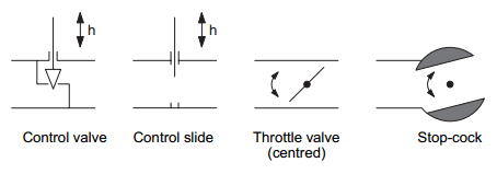
Picture 1: Final control elements in flow technology
Picture 2 therefore illustrates the design of a control valve (schematic), whereby an equivalent electrical circuit diagram is also provided to facilitate any possible similar considerations (Picture 3).

Picture 2: Design of a control valve
Faced with the task of selecting a final control element, the first step is to examine the basic behaviour of the final control element in a system section (pipe section). In this context, it should be noted that due to the flow resistance of this final control element, a dynamic pressure drop occurs ∆p, which quadratically depends on the flow velocity or throughput. This means that part of the overall pressure available at the start of the pipe is reduced in the final control element (loss of energy).

Picture 3: Equivalent electrical circuit diagram of a control valve
Due to its nature, it follows that a process technological system will always be equipped with numerous control valves, in that different flow and pressure conditions will occur. It is therefore necessary to introduce the main parameters and facts in order to classify these control valves. To be able to make a permanently (experimentally) reproducible comparison of control valves, manufacturers work on the basis of a standard state (standard flow rate) of the valve to be used and define the so-called kv value. This means that for a pressure drop of 0.98 bar (0.98 − 105Pa), manufacturers specify water flow rates of (ρ = 103 kg/m3) passing through the valve. These standard flow rates depend purely on the valve stroke y and are referred to as kv value. The throughput associated with the nominal stroke of the control valve is known as kvs value.
The dependency of the kv values on the respective valve stroke is recorded in the so-called steady-state characteristic curve or basic characteristic curve of the control valve. The most typical basic forms of this basic characteristic curve can be most frequently found in:
>> the linear characteristic curve (a variation of valve stroke causes a change in linear throughput – see Picture 4);
>> the equal-percentage characteristic curve (variation of valve stroke and throughput have a non-linear correlation – see Picture 4).

Picture 4: Basic characteristic curve of control valves
On the basis of the actual automation task (design of process technological system section) it has to be decided, which basic characteristic curve is to be used. To give a practical indication, the following procedure can be recommended:
If the static characteristic curve is known (estimation) for the process technological section intended for the use of the valve, then the basic characteristic curve of the control valve is to be selected in such a way that, with the added superimposing of both characteristic curves (with the interaction of system section, and control valve) a as near as possible linear steady state characteristic curve (operating characteristics) is obtained for the flow behaviour.
Furthermore, it should be noted that various control valves, depending on the constructional design, do not completely seal during a zero valve stroke. The resulting residual throughput is referred as the kVo value of the control valve. From the point of view of cost and function, this should not necessarily be regarded as a disadvantage, since the comparatively simple On/Off valves are often used to completely close off pipes. Moreover, the control valve can be fashioned into a completely closing version by means of corresponding design changes (e. g. use of compressible seals). In this case, one also speaks of the so-called zero-point suppression. In this case, the characteristic curve greatly deviates from the actual basic characteristic curve in the case of a small stroke (Picture 5).

Picture 5: Linear basic characteristic curves of control valves with and without zero suppression
The parameters kvs and kvo are used to form the so-called theoretical control ratio kvs/kvo, which is generally specified as a typical parameter by the valve manufacturer and, in practice is often also replaced by the effective control ratio kvs/kvr. This takes into account the tolerance between the targeted and the actually measured basic characteristic curve (see also Picture 5).
If we now turn to the impending valve selection then, according to the above information, we start with the kv value. For a pressure drop ∆p≈1bar (specification resulting from practical experience) this can be determined as follows by the project engineer, taking into account the flow rate of the system section (specification resulting from practical experience:
Kv = 0.032 * q * √(ρ/∆p)
q – Output flow in m3/h (flow rate);
ρ – Density of passing medium in 103kg/m3;
∆p – Pressure drop via control valve (specification 1 bar).
This means that by defining (estimating) the maximum and minimum flow rates (qmax/qmin) in the system section in question, the following characteristic values are calculated with the help of the above formula:
kvs = 0.032 * qmax * √(ρ/∆p)
(maximum valve stroke y/ also Kv max) and
Kvmin = 0.032 * qmin * √(ρ/∆p)
(minimum valve stroke y).
For practical purposes, it should be noted that, in most cases it is not possible to find a control valve with the kvs value calculated from the system data. Consequently, for practical reasons, (e. g. also taking into account any other occurring changes in the system data) one should always select a control valve with a higher kvs value (than that calculated), i.e. the control ratio kvs/kvr.
Additionally, it should be mentioned that by changing the formula to determine the kv value, it is also possible to obtain a formula for the above mentioned operating characteristics, which is as follows:
q = kv * 31.62 * √(∆p/ρ) = g (y, ∆p)
However, in this case ∆p represents the actual pressure drop via the control valve for the respective flow rate, which can only be recorded metrologically, but in practice is not realised in the form of a measuring point. The formula is therefore less relevant in practical terms and the satisfactory (practically linear) operating characteristic can only be achieved by means of the already mentioned superimposition of basic characteristic curve and system characteristic curve. In conclusion, a few comments should also be added with regard to the classification /estimation of the steady-state characteristic curves of process technology system groups. As can be seen from Picture 8, differentiation is made between system sections with dominant static pressure drop and dominant dynamic pressure drop. However, in Picture 6, it can be clearly seen that in systems with static pressure drop, this only marginally depends on the flow rate, also known as output flow q.

Picture 6: System with steady-state pressure drop (ideal case – pump resistance neglected)
It therefore generally applies that the overall pressure drop remains constant and as such also the pressure drops via the system section and control valve. In the case of system sections with dynamic pressure drop, the pressure changes in relation to the output flow q and via the system section itself, and via the control valve as per Picture 7.

Picture 7: System section with dynamic pressure drop (ideal case – pump resistance neglected)
Picture 8 represents a summary of the main considerations involved in selecting a control valve, which are documented in the form of basic rules of procedure via points 1 to 4.

Picture 8: Selection of a control valve
Selection of sensors
As a rule, the selection of sensors within the framework of an automation project is more straightforward than the selection of actuators described in the last section. The selection by means of evaluating the respective company literature is relatively simple for the project engineer. By using the measuring ranges associated with process technology, all that remains for him to do is to select a corresponding sensor. Picture 9 illustrates this procedure. Needless to say, the environmental operating conditions of the sensor also are to be taken into account (e. g. aggressive medium, assembly conditions, etc.).

Picture 9: Selection of sensors
No comments:
Post a Comment