The temperature control system of the small-scale experimental modules in the experimental state consists of an electrically heatable container, in which the water temperature in increased (Picture 1). To obtain a better distribution of temperature in the container, the water can be agitated by means of a centrifugal pump. This results in constant thorough mixing, which prevents the formation of differing heat levels. The purpose of the automation task is to control the water temperature T (controlled variable) by means of the heat output Pel (correcting variable). The special characteristic of this controlled system is that the temperature is lowered solely as a result of heat dissipated to the environment. The output of this process, i. e. the heat dissipation ∆Qout in the time interval ∆t, is considerably less compared to the maximum heat output.
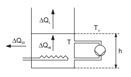
Picture 1: Schematic representation of temperature control system
The following abbreviations mean:
>> T - Water temperature in the container;
>> Tu - Ambient temperature (air);
>> ∆Qel - Quantity of heat output by heater system in ∆t;
>> ∆QL - Quantity of heat emitted directly to air in ∆t;
>> ∆QW - Quantity of heat emitted through wall in ∆t;
>> h - Filling level in container.
Theoretical model configuration
The heating process in the temperature control system can be represented in a greatly simplified manner as follows (Picture 2).

Picture 2: Simplified representation of temperature control system
The following mean:
>> V = c * m * T – internal energy of volume of water with m = ρV = ρ * A * h;
>> ∆Qel = Pel * ∆t – quantity of heat output via heating system in time interval ∆t;
>> ∆QL = α * AL * (T − Tu) * ∆t – quantity of heat (heat transmission) directly emitted to the air via the exposed water level in ∆t;
>> α – heat transmission coefficient (water – air);
>> ∆QW = k * AW * (T − Tu) * ∆t – quantity of heat (heat transmission) emitted to the air via the wall in ∆t;
>> k – heat transmission coefficient (water – container wall – air).
The quantity of heat supplied and removed during time interval ∆t, can be noted as follows:
∆Qin = Pel * ∆t or
∆Qout = ∆QW + ∆QL
The temperature T only changes if a difference ∆Q occurs between the quantities of heat:
∆Q = ∆Qzu − ∆Qab
This difference is the change of the internal energy of the volume of water:
∆Q = ∆U = c * m * ∆T
Steady-state model of closed control loop
The supplied and removed quantities of heat must coincide in the stationary state (∆Q = const., ∆T = const.):
∆Qin = ∆Qout
and hence
Pel = α * AL * (T − Tu) + k * AW * (T − Tu)
must apply. With an assumed constant ambient temperature, this equation results in the correlation
T (Pel) = Pel/(α * AL + k * Aw) + Tu
which indicates the dependence between heating capacity output and water temperature in the stationary state. Picture 3 shows the steady-state characteristic curve of the temperature control system. An assumed constant ambient temperature becomes less and less valid with increased heat dissipation. With increasing ambient temperature, the lost heat flow decreases, (∆Qab ~ T-Tu), whereby the water temperature becomes higher than in the ideal case.
The heating module used can be actuated intermittently, since it is either switched on at full capacity or switched off completely (two-point element). Any desired heat output can be achieved by means of periodic switching on or off of the heating module. The periodic time tper is used to calculate the output from the switch-on time ton and the heat output in the switched on status Pelmax at:
Pel = Pel max * ton/tper

Picture 3: Qualitative process of steady-state characteristic curve of temperature control system (ideal case)
The periodic time tper must be sufficiently long so as not to excessively load the contactor in the control head in the heater modules as a result of frequent switching. On the other hand, the periodic time selected must be short, so that the temperature pattern remains even (Picture 4). This means that is must be considerably shorter than the controlled system time constant of the heating or cooling process (e. g. tper = 10 s).

Picture 4: Temperature and performance pattern during on/off switching of heater module (two-point element)
Linear dynamic controlled system model
If we now look at the following equation again:
∆Qin − ∆Qout = c * m * ∆T
and apply this for the supplied and dissipated quantity of heat, this results in the following correlation for the temperature change ∆T per time interval:
∆T/∆t = [1/(c * m)] * [Pel − (α * AL + k * AW) * (T − Tu)]
This controlled system section represents a sufficiently small ∆t selected, and is the basis of the behaviour shown in Picture 5 (a). The temperature control system therefore has a proportional action with a delay of the first order. The change in heat output causes a gradual temperature change.
Again, it should be pointed out that the rate of change in temperature is not the same for heating and cooling. Picture 5 shows the qualitative pattern of the two processes. In addition, a considerably shorter dead time Tt occurs in the case of heating compared to the system time constant THeating. This is caused by the heat capacity of the heater module and the heat conduction speed in the water. This latter time constant can be lowered by moving or stirring the water. The parameters K, THeating and TCooling are to be determined by experiment.

Picture 5: Qualitative representation of system step response: a) Heating b) Cooling
No comments:
Post a Comment