Control algorithms
Control algorithms have proved to be a tried and tested method of calculating the correcting variable Y from the system deviation e, which relates back to the basic behaviour patterns of the response characteristic (P-, I-, D-action) of technical systems. Each action assumes its own particular role in the course of this processing of information. Picture 1 shows the signal flow diagram (the graphic representation of signal processing) of the controller. The purpose of P and D-action is to ensure an as quick as possible but smooth process of the transient phenomenon in closed control loops. The D-action does not have any effect on the stationary state of a closed control loop, since even with a steady-state deviation es (τµ) 0, the output signal YD decays towards zero and therefore does not contribute towards the stationary value of the control signal Y. However, the effect of this action comes into force particularly quickly with variable system deviations. To some degree, the D-action therefore contributes in advance, i.e. in anticipatory manner to the control signal Y. The actual action function is to keep the controller characteristic curve vertical and thus to completely correct any permanent interference. This relates to the previously illustrated characteristic of integral-action systems to generate a constant rate of change of the system output variable after a jump activation. This is how the system output (in the case of the controller, the signal Y) can assume any I value within its control range, even though the input signal (in this case the system deviation e) attains the value zero again after a transient response. An integral action system therefore has a steady-state effect in the same way as a proportionally acting system with infinitely significant proportional coefficient. Over a sufficiently long period of time, the smallest uni-dimensional input signal values lead to an output signal of some significance. In order to be able to calculate the overall effect of the controller on the closed control loop behaviour and as such the time-related response of controlled variables X and Y in relation to the task, the controller actions can be introduced into the calculation of the values of setpoint specification Y. For this, every PID controllers has three freely adjustable parameters (characteristic controller values):
>> the proportional coefficient KR for the adjustment of the P-action;
>> the correction time Tn for the adjustment of the I-action;
>> the derivative-action time Tv for the adjustment of the D-action.
Dynamic closed control loop behaviour requirements
The adjustment of the characteristic controller values KR, Tn and Tv largely depends on:
>> the steady-state and dynamic behaviour of the controlled system;
>> the disturbances acting on the controlled system;
>> the demands placed on the steady-state and dynamic behaviour of the closed control loop.
The steady-state behaviour of the closed control loop (working point setting, steady-state system deviation, functions and effect of the I-action in the controller) has already been described in detail in the section Steady-state behaviour of the closed control loop in Controller Configuration and Parameterisation.
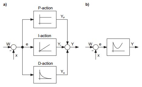
Picture 1: Signal flow diagram of PID-controller:
a) with individual representation of controller actions P, I and D
b) with overall representation (Addition of individual representations) of controller transient function hR(t)
The same preconditions should be assumed for the discussion of the dynamic behaviour as those applied for the linear dynamic model of technical systems. Here, it is assumed that all process signals during the control processes occur in the vicinity of their working points and do not in practice deviate from the linearity range. In this way, the demands placed on the dynamic behaviour of the closed control loop, e. g. in the form of step responses can be precisely defined. However, this means that during the practical operation of the closed control loop, the boundaries of the linear working range around the working point must be observed. If these are exceeded, then the results achievable in this case with the controller settings based on the linear dynamic models are also called into question.
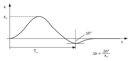
Picture 2 illustrates a behaviour of the controlled variable x(t) after the sudden change of the setpoint value w (control step response of the closed control loop), which should be aimed for. This behaviour can be described roughly by two characteristic values:
>> the overshoot time Tm;
>> the standardised overshoot amplitude ∆h = ∆h∗ / w.
The overshoot amplitude ∆h usually requires a value between 0 and 20 %t. Overshoot time requirements Tm depend on the dynamic behaviour of the closed control loop and must always be viewed in conjunction with the process dead times and process constants. If the inflectional tangent model introduced in the section The inflectional tangent model in The Inflectional Tangent & The Total Time Constant model is used to describe the controlled system behaviour, then the overshoot time should not be less than half the total of the time delay and the transient time specified (reference value). This ensures that the control signal y does not assume untenably high values during the transient stage.

Picture 2: Favourable behaviour of control step response of a closed control loop
A similar process can be adopted with regard to a favourable course of the interference step response of the closed control loop (step-change response of the closed control loop at its input). Picture 3 shows a favourable course of this process from the control technology viewpoint.
Picture 3: Favourable behaviour of interference step response of a closed control loop
Here too, the process can be described roughly by means of two characteristic values (Tm and ∆h* or xm).
No comments:
Post a Comment