In automation technology, calculation models (behaviour models in the narrower sense) are primarily used, which quantitatively describe the main relationships between process variables, e. g. in the form of mathematical correlations, characteristic functions, performance data, etc. Picture 1 illustrates the basic structure of this form of model, where:
>> y – correcting variable;
>> z – main disturbance variable;
>> v – negligible disturbance variable;
>> x – output variable.

Picture 1: Basic structure of calculation models
This provides an initial illustration of the line of action of the process signals, without the sometimes complicated "process content". Moreover, it is assumed that all process variables (e. g. flow rate, temperature, filling level, etc.) are dependent merely on time, but not on location (such as in the case of process technology systems of significant physical dimensions). In accordance with Picture 1, the calculation models now have to quantitatively represent the dependence of the output variable x on the input variable y, z and possibly also v, whereby a differentiation should be made here between static and dynamic models.
The relationship between the input and the output variables of a technical system in its steady-state condition is known as the static behaviour. A simple example of this is shown in Picture 2, in the form of a so-called correcting characteristic of a controlled system, i.e. the relationship between, for example, the valve position y as a process input variable and the temperature x as a process output variable with the main interference z (e. g. pressure) as a performance data parameter.
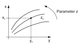
Picture 2: Control characteristic curve in the form of steady-state model
The index zero designates the working point values (process signal values during nominal operation). However, input and output signals change from time to time during the operation of technical equipment, due to starting and shut down procedures and varying, unforeseeable disturbances. This is why it is often essential for the process model to include the description of the relationship between these time-related signal changes, which is also known as dynamic behaviour. Dynamic models in the form of linear models are often adequate, even for example for the important task of process stabilisation with the help of a closed control loop. This is possible in cases where the process signals operate sufficiently closely to the working point during the execution of technical processes, so that the process behaviour does not perceptibly change even during transitional phases. In the case of practical operation of automation equipment, it then becomes necessary to consider the limits of the linear operating range. If these are exceeded, then the results achievable in the course of the system design using the linear models are put into question.
Model configuration through experimental process analysis
The following describes the procedure of experimental model configuration in greater detail. The main feature of this is that, with the help of suitable experimental technology, the analyses are carried out immediately on the technical system and the data obtained can be converted into a process model graded according to different levels (starting with the simple manual analysis method through to computer assisted data evaluation) (Picture 3).

Picture 3: Basic structure for experimental process analysis
The main points and problems of an experimental process analysis consists of:
>> the formulation of requirements demanded of the model (application aim, accuracy, validity range);
>> the preparation and implementation of the experiments;
>> the selection of suitable methods for the analysis of the process data recorded;
>> error estimation and model verification.
As part or the preliminary stage of the experiment, the following should be considered:
>> the auxiliary hardware and software devices;
>> the model structure (e. g. in the form of qualitative information regarding the process behaviour);
>> the main process influencing variables, in particular also the disturbance variables;
>> the required measuring times.
The hardware and metrology preparations include:
>> the assembly of suitable control, measuring and recording techniques, unless already available on the process;
>> the verification of the experimental techniques/technology under operating conditions.
As part of the experiments, it is often necessary to carry out preliminary experiments in order to establish modulation ranges, adequate signalto-disturbance ratio and main influencing variables. With the main experiments it is important to ensure that sufficient data material is registered to determine the working point values (initial values at start of measurement). Useful signals at the system output must have sufficient noise ratio; in the case of experiments with step-type input signals, they should therefore be modified by approximately 10 % of their correcting range (caution: observe linearity range!). Picture 4 shows an example of the undisturbed (theoretical), i.e. faulty (determined during practical operation) step response x(t) of a technical system. A simple quantitative measure of the signal/disturbance ratio is the amplitude ratio
S = AS/AN
of disturbance signal and useful signal in the steady-state condition.

Picture 4: Illustration of disturbance/useful signal ratio using the example of a faulty step response
No comments:
Post a Comment