The Michelson-Morley paradox solved


The Michelson-Morley Paradox Solved is a treatise written by Justin Jacobs. It thoroughly examines the Michelson-Morley paradoxical null results and is written in a manner that is meant to make it approachable to the general public. In this article we expose the whole Section 8 of this treatise, which is the section where the author describes the main idea of its treatise.


THE REAL AND CORRECT THEORETICAL, EMPIRICAL & TECHNICAL SOLUTIONS FOR MICHELSON’S PARADOXICAL NULL RESULTS


The first real reason for Michelson’s null results is completely theoretical. Michelson was attempting to detect the absolute velocity of the Earth through the ether by detecting a theoretical difference between two theoretical time intervals for light rays to propagate in two different directions, with respect to the ether.

There were at least nine different ether theories concerning the theoretical difference in time intervals, or why such difference was not detected:
1) Lorentz’s 1886 stationary ether theory;
2) Fresnel’s 1818 theory that the ether was being partially dragged along by the Earth;
3) George Stokes’ 1845 theory that the ether was being totally dragged along by the Earth’s motion through it;
4) Maxwell’s 1879 ether displacement theory which compared light propagation on a moving Earth and on an absolutely stationary Earth;
5) the “ether wind” theory which should decrease the velocity of light in the direction of the Earth’s solar orbital motion;
6) Michelson’s theory that the longitudinal mirror in his apparatus would displace from stationary ether and a propagating light ray in the direction of the Earth’s solar orbital motion;
7) Michelson & Morley’s theory that both mirrors in their apparatus should be displacing differently from stationary ether;
8) Fitzgerald’s and Lorentz’s theory that the time interval difference existed but it could not be detected because of a physical contraction of matter; and
9) Einstein’s theory that the difference in time intervals should result from the way time coordinates are measured.
Theoretically, several of these different ether theories should have produced a specific time interval difference for light to propagate in a certain direction. But Michelson never detected any difference in the time interval for light to propagate in any different direction of the Earth’s motion through space, nor has anyone else.


Apparently, no one has ever realized that all of these absolute theories and theoretical positions, motions, dragging effects, displacements of mirrors, decreases in the speed of light, distance intervals and time intervals of light propagation, measurements of time coordinates, and mathematical calculations of the same, and many absolute expectations were based on one completely false and impossible assumption: the existence of a material substance called ether.

Since we now know that the concept of ether (stationary, dragged along, or otherwise) was only a manmade myth and does not exist, therefore the absolute place or position from which all of these theories, measurements, and computations were made or described also does not exist. In reality, all of these illusionary theories, “measurements,” “computations,” and expectations were made with respect to “nothing. As George Gamow stated in his 1961 book, “One cannot move with respect to nothing…one can speak only about the relative motion of a material body in respect to another [material body].” It also follows that one also cannot measure, describe, or calculate something with respect to nothing. In this regard, let us also quote from Richard Feynman,

“You can only define what you can measure! Since it is self-evident that one cannot measure a velocity without seeing what he is measuring it relative to, therefore it is clear that there is no meaning to absolute velocity. The physicists should have realized that they can talk only about what they can measure.”

These were the fundamental theoretical reasons why Michelson could not detect a greater distance/time interval for light to propagate in the absolute direction of the Earth’s solar orbital motion through space, or in any other absolute direction of the Earth’s motion through space. There was never anything to detect! Such a greater or increasing distance/time interval for light to propagate in any direction with respect to nothing simply does not exist. It was yet another ether myth. It is also self-evident that Michelson, Morley, Kennedy, Thorndike, and anyone else cannot detect (by any method) a time interval difference that does not exist. Their elaborate efforts to do so were always an absolutely meaningless mission impossible!

There was also another related theoretical problem: Michelson’s experiments, the Kennedy-Thorndike experiments, repetitions thereof, and similar experiments were always assumed, described, interpreted, and believed to have resulted in “null results,” because completely different results were absolutely expected. However, all of these so-called null results actually resulted in empirically positive results, again because there was nothing to detect.

There was no difference in “time intervals for light propagation through ether or space,” that could be detected. There was no greater distance or time interval for light to propagate between relatively stationary mirrors in any direction of the Earth’s motion through ether or space that could be detected. There was no decrease in the velocity of light in the direction of the Earth’s motion through ether that could be detected. There was no displacement of mirrors from a propagating light ray in the direction of the Earth’s solar orbital motion, through the ether that could be detected. The reason for all of these factors is that there is no such thing as stationary ether, ether wind, or dragged along ether which could be detected either.

The scientific community simply refused to believe in all of these empirical results, and it still does. There is a huge lesson to be learned from these unscientific facts. That is: always believe in and trust reasonable physical observations and empirical results over illogical theoretical expectations, unobserved theoretical phenomena, and over mathematical theories, equations and computations.

The real reason why there was no change in the velocity of light in any direction of the Earth’s motion through space is because the light rays propagating in Michelson’s and Kennedy’s experiments always propagated through the same medium: clear air. It is well known from the Index of Refraction that light always propagates through clear air at sea level at almost velocity c (only 0.0003 less fast). This is also the real reason why light was always detected to be c in every light experiment conducted in any inertial frame of reference on Earth, or in space.

The next real reason for Michelson’s null results is physical and empirical. Let us postulate that the finite physical distance between two relatively stationary physical points (A and B) does not change just because such two points move in-tandem through space in any particular direction. Such finite distance between A and B always retains the same finite magnitude101 (Picture 1). The positive empirical results of Michelson’s and Kennedy’s experiments described this postulate, because no fringe shift was ever detected during either experiment.

In addition, let us also postulate that a light ray can only propagate at the constant velocity of c over any finite physical distance through the vacuum of space (or air), and that the velocity of such light ray at c does not change just because it propagates through the vacuum of space (or air) in any particular direction102 (Picture 1). The positive empirical results of Michelson’s and Kennedy’s experiments also described this postulate, because no fringe shift was ever detected during either experiment.


Picture 1: Light Measured At Velocity c To And From On Two Different Reference Frames


The fundamental reason for the last above postulate is because the medium (i.e. the vacuum or the air) through which the light ray is transmitting in Picture 1, is the primary determining factor for the velocity of the propagating light ray, and the medium never changed in either experiment. Light always transmits through a vacuum at the constant velocity of c (300,000 km/s, the fastest speed that nature allows), because there are no particles of matter in a perfect vacuum to slow light down or change its direction of transmission.

The velocity of the vehicle in which the light experiment is traveling has nothing to do with the velocity of the light ray within the vehicle. For example, if one of the vehicles in Picture 1 was filled with water the light ray would propagate much slower in that vehicle (about 225,000 km/s). The confirmation of these facts is the empirical index of refraction where light propagates at different velocities through different media.

Because of these above described postulates, there can never be an increasing physical distance or a greater time interval for light to propagate between two relatively stationary physical points (A and B), regardless of their in-tandem motion through the vacuum of empty space in any direction. Therefore, these postulates demonstrate the empirical validity of Michelson’s and Kennedy’s results. There never was a greater time interval for light to propagate within Michelson’s or Kennedy’s apparatus in any direction. These results have been demonstrated many times in many different reference frames.

Another real, physical and empirical reason for Michelson’s so-called null results, which apparently has been completely overlooked by everyone, was that M & M were actually only attempting to measure (or compare) one slightly out-of-phase light wave relative to another slightly out-of-phase light wave (Picture 2). Such out-of-phase light waves created an interference fringe when Michelson slightly changed the distance of one mirror by fine tuning its micrometer screw. M & M then assumed that the solar orbital motion of the Earth would change the distance/time interval which one light wave would have to propagate away from the ether. But, to paraphrase Feynman, one can only assume that which one can measure, and one can only measure that which one can see. One cannot measure unobserved or undetectable phenomena.
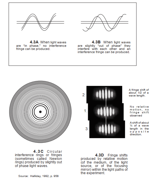


Picture 2: Out Of Phase Light Waves Can Create An Interference Fringe, And Relative Motion Within The Light Paths Of The Experiment Can Create Fringe Shifts


Regardless of what M & M were assuming, and regardless of the direction that their apparatus might be pointing in, if the finite physical distance of each arm of his apparatus always remained the same, there could never physically be an interference fringe shift: that is, a change of the relative phase positions of such out-of-phase light waves. Stated somewhat differently: As long as the physical length of each arm did not change (whatever its magnitude of distance might be), the relative phase position of each out-of-phase light wave would physically have to remain the same. This was the empirical result of the 1932 Kennedy-Thorndike experiment where one arm was intentionally constructed much shorter in length than the other arm (Picture 3). Therefore, the specific finite length of each arm and the specific finite distance that each light ray propagated in any direction were always irrelevant to the occurrence of a fringe shift.


Picture 3: The 1932 Kennedy-Thorndike Experiment


For all of the above real, physical and empirical reasons, a fringe shift could never physically occur when Michelson or Kennedy pointed the arms of his apparatus in different directions over a period of several months. Michelson’s and Kennedy’s attempts to detect an interference fringe shift, or a difference in time intervals for light propagation in any direction, were always a mission impossible. In order to visualize what actually happened in Michelson’s experiments, refer to Picture 4.


Picture 4: Two Perpendicular Light Pencils Propagating Within Michelson’s Apparatus At 4 Different Times, In The Absence Of Stationary Ether


The next real reasons for Michelson’s null results are technical. We have already described one of these technical reasons. If the arms of Michelson’s and Kennedy’s experiments always remained the same finite length, then a fringe shift (a change in the relative phase position of two slightly out-of-phase light waves) never could have physically occurred (Pictures 3 and 5). The only way that a fringe shift could have occurred would be if Michelson or Kennedy would have slightly adjusted the distance of the focusing mirror with the micrometer screw in order to obtain a fringe (Picture 6). But since both scientists already had obtained an interference fringe, there was no reason for them to obtain another one. And they never did.


Picture 5: Michelson’s Interference of Light Experiments


Picture 6: What Happened When Michelson Adjusted The Distance Of One Mirror In The Path Of One Light Pencil?


A second technical reason was because M & M’s apparatus was located in the concrete basement of a building (with no windows) so that its sensitive instruments would not be affected by traffic, heat, sunlight, etc. If M & M had desired to visually detect the motion of the Earth’s solar orbital motion, or any other relative motion of the Earth, they could have mounted a 10-inch telescope on the roof of the building and observed the light paths of a passing luminous planet (i.e. Venus) or a luminous planet that the Earth was passing (i.e. Mars, Jupiter, or Saturn) through the lens of the telescope and calculated the solar orbital motion of the Earth over a period of months.

However, the solar orbital motion of the Earth could never be detected by the interference method employed by M & M or Kennedy & Thorndike from the basement of a building, because (unlike the telescope) there never was any material body which moved within the light paths of their interference experiment, which technically could be detected by any method. The only motion which occurred within the light paths of their experiments was when the focusing mirror was adjusted by the micrometer screw to create an interference fringe. For this simple technical reason, none of these scientists could ever detect anything else, and none of them ever did.


Source: The Michelson-Morley paradox solved (You can also read the whole treatise there)

The Experiment of Fizeau


The short description of the experiment of Fizeau:

1. When the water is not moving in each tube, the light propagating through each tube has the same velocity, so the light waves in the two pencils of light that reach the eye are in phase.

2. When light propagates through water moving in different directions at 7 m/s, the velocity of light relative to the tube increases in the direction of flow A and decreases in the opposite direction of flow B. Thus the light waves propagating through tube A will arrive at the eye sooner (and in less time) than the light waves propagating through tube B. This causes an out of phase interference of the crests and troughs of such light waves which is visible to the eye as a pattern of interference fringes. The distance between each dark fringe is one wave length.


Picture 1: The experiment of Fizeau which determined the velocity of light in a moving liquid

When the flow of the water in the tubes is reversed, the pattern of interference fringes shifts, and the measurable magnitude of this shift can be computed to determine the difference in the velocity of light propagating relative to each tube.

Maxwell’s 1879 Ether Assumptions


Picture 1: Light propagating in any direction on the theoretically stationary Earth


The Picture 1 also illustrates Michelson’s theoretical distance and time interval (T1) for light to propagate in the direction perpendicular to the Earth’s solar orbital motion.


Picture 2: Light propagating in the direction of Earth’s absolute solar orbital motion and away from the stationary ether


The Picture 2 also illustrates the theoretical in-tandem displacement of mirrors A and B with respect to the stationary ether. Because empirically there is no ether, these theoretical displacements from ether cannot occur.

The light source, the beam splitter (BS) and the mirror M are affixed to the surface of the Earth at a finite distance apart, and for purposes of illustration we assume that they move in tandem to the right at 50% of c relative to the stationary ether and the Sun theoretically at rest in the ether. A light ray leaves the terrestrial light source at some point A0 and transmits at 100% of c toward the mirror at some point M0. During such propagation, the mirror theoretically displaces from point M0 to some point M1 due to such absolute solar orbital velocity with respect to the stationary ether. The light ray contacts the mirror at point M1 after traveling (from A0 to M1). The light ray then reflects from the mirror at M1 and begins to propagate back toward the light source. During such propagation, the material light source theoretically displaces from point A0 to some point A1 and then to some point A2.
When the light ray returns to the light source at point A2 the light ray has traveled a total distance/time interval while the light source and the mirrors have theoretically displaced in-tandem 1/2 of the total distance, an increase of 1/4 of the total distance because of the theoretical displacement. These were also Einstein’s computations for a greater distance/time interval of light propagation, which he referred to in Relativity at pp. 58 - 59. On the other hand, if there had been no motion of the Earth in an absolute direction(and thus no absolute displacement), then the light ray would only have traveled a total distance/time interval of 3/4 of the total distance. Strangely enough is what actually happened, because there is no ether and there can be no physical displacement from something that does not exist.

Astable Oscillator Circuit with 555 Timer


As we already analyze one simple Astable circuit with 555 Timer, now we will analyze one improved circuit with the same 555 timer. The oscillator circuit is shown on Picture 1. The main difference in this circuit is that resistor R3 now is connected to the trigger pin of the 555 timer and to the output of the circuit via the capacitor C3.


Picture 1: Astable oscillator circuit with 555 Timer


Time-domain analysis


The results of the transient analysis for this circuit in time domain is shown on Picture 2. These results are for the configuration of the circuit as shown on Picture 1. The power supply voltage is Vcc = 5 V DC. Resistor R3 = 270 Ω, R1 = R2 = 500 Ω, while the capacitors are C1 = 100 nF and C2 = C3 = 1 nF. As measured in the simulation, the frequency of the output signal is about f = 1.826 MHz.


Picture 2: Transient analysis - output voltage Vo wave form (time-domain)


The frequency of the output signal of this circuit can be changed, if we change the values of the components of the circuit. For example, we run simulations with three different values for resistors R1 and R2, and we got these results:

>> For R1 = R2 = 500 Ω -> f = 1.826 MHz;
>> For R1 = R2 = 820 Ω -> f = 1.662 MHz;
>> For R1 = R2 = 1 KΩ -> f = 1.632 MHz;


Just to notice here, the model of the NE555 timer circuit used in these simulations is idealised. In practice, this circuit has some upper limit for frequency of operation. This limit depends on the model and technology of the manufactured circuit. Usually, the older circuits had limit below 1 MHz, but the newer 555 Timers can have upper limit frequency of few MHz-s. Above the upper limit the circuit will be unstable.

Modulators and Feedback


There are numerous modulators, and here it is not objective to give an extensive overview, only the basic topologies are discussed.


PDM modulators


PDM modulators have resulted from the digital signal processing domain. In more and more equipment, the signal is available in digital form. For a switching amplifier it must be converted into a 1 bit signal at a high frequency. Sometimes, as with DSD audio data, this is even the native format. The output stage acts as a 1 bit D/A converter. Because the length of each bit is constant, and only the presence or non-presence of a bit is controlled, this is called Pulse Density Modulation (PDM). To convert a multi-bit signal to a 1-bit signal, oversampled noise shaping is used. Picture 1 shows a general noise shaper.


Picture 1: Noise shaper


The input signal Bin(z) has a larger number of bits than Bout(z). (When the input signal is analogue, a similar structure in the analogue domain constitutes a sigma-delta modulator). The block called "Quantizer" reduces the number of bits by simply passing only the most significant bits to Bout(z). The least significant bits, which are the error, are added to the input after passing through a transfer function J(z). It is easy to calculate Bout:

Bout(z) = Bin(z) - ε(z)(1 - J(z))

Suppose J(z) = z-1, one clock delay. The system is now a first-order noise shaper. Bin(z) is a 16 bit signal at 256fs and Bout is a 1 bit signal at 256fs. In that case, the quantizer transfers 1 bit to the output. The other 15 bits are the error signal. Bout equals:

Bout(z) = Bin(z) - ε(z)(1 - z^-1)

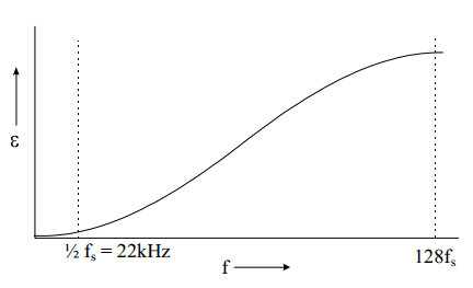
With z = e^( 2πj(f/256fs)), we see that for low frequencies (audio) the error in the output signal approaches zero. The error reaches a maximum for f = 128fs. See Picture 2.


Picture 2: Noise distribution as a function of frequency


Applying Bout to a 1 bit D/A converter and filtering above 20 kHz reconstructs the original signal. In the time domain such a noise shaper is a way to convert resolution in the amplitude domain to resolution in the time domain. It outputs bits at high speed in such a way that the average is the intended output (which has a higher amplitude resolution). This way it is also easy to see that although the D/A converter is only 1 bit, it should have a 16 bit accuracy.
To convert the audio signal to 256fs, an oversampling interpolating filter must proceed the noise shaper. A two times oversampling filter works as follows. Suppose the spectrum of the signal sampled at fs looks like Picture 3. This signal is converted to a sampling frequency of 2fs by inserting a sample of value zero after every original sample. See Picture 4. Because every sample is a Dirac pulse of proportional height, the frequency spectrum stays exactly the same.


Picture 3: Spectrum of the signal


Picture 4: Inserting zero samples


Next, the signal is applied to a digital filter at 2fs that filters out the middle replica, see Picture 5. After that, the frequency spectrum of the signal looks exactly like it has been sampled at 2fs. These techniques, oversampling interpolating filtering and noise shaping are essential for all digital PDM systems, although the exact realisation may vary.


Picture 5: Filtering out the middle replica


Assume, the 256 times oversampling for a CD player D/A converter is done in two stages. A four times oversampling filter is followed by a 64 times linear interpolator. The direct use of a 256 times oversampling filter is also possible, but the filter would be very large. A linearly interpolating filter is easier to build, and at 4fs the distortion that it creates has only little effect in the audio band. Then, at 256fs, a second order noise shaper suffices to get a 1 bit signal with 16 bit resolution in the audio band. Unfortunately 256fs = 11MHz which is too high for power switching.
Another possibility is to use only 32fs with an eighth order noise shaper.
Noise shapers with a higher order than three are prone to instability, and it is necessary to manipulate the system when it becomes potentially unstable. Extensive simulations are necessary for evaluation. Even in this case, the switching frequency is 1.4 MHz. The high switching frequencies are a general problem of PDM modulators. Bit-flipping techniques can reduce the average frequency at which the output changes somewhat.


Digital PWM modulators


Digital PWM modulators offer a lower switching frequency than PDM modulators. The Pulse Amplitude Modulated (PAM) samples are converted to PWM. This could be done by giving each pulse a length that is proportional to the original amplitude. However, for CD quality the internal clock frequency would have
to be 2^16 * 44.1 kHz = 2.9 GHz, which is way too high. Furthermore, the frequency spectrum of the PWM signal would not equal that of the PAM signal. This can be calculated, but for a better understanding it is best to realise that natural sampling yields the best results because it does not introduce harmonic distortion. In natural sampling, the audio signal is compared to a triangle or sawtooth waveform (more details below). When we convert a digital PAM signal directly to PWM, it looks as if, looking in the analogue domain, we compared the sawtooth waveform to a step-like representation of the signal instead of the signal itself. This is called uniform sampling. See Picture 6. It introduces harmonic distortion, which depends on many factors including the signal frequency, the switching frequency and the modulation depth.


Picture 6: Natural sampling versus uniform sampling


To approximate natural sampling, linear or higher order interpolation between two or more samples is used to approach the natural PWM pulse width. When the pulse width has been calculated, the sample instant can be the beginning or the end of the pulse (single sided modulation) or the middle (double sided modulation). There are more aspects that deserve attention, but a full discussion of these would be beyond the scope of this article.


Analogue PWM modulators


In the analogue domain a PWM signal can be generated by comparing the audio signal to a triangle or sawtooth waveform. This technique, called natural sampling, is the basis of almost all analogue modulators. See Picture 7. When the momentary value of the input signal is larger than the triangle, the output of the switch is high. It is easy to see that in this way the pulse width at the output is proportional to the input voltage. The modulator does not introduce harmonic distortion, only (multiples of) the carrier frequency and (multiples of) harmonics of the modulating frequency around the carrier.


Picture 7: Open-loop class D modulator


The main problem is the lack of feedback. Output stage inaccuracies, nonlinearities, timing errors and supply voltage variations all contribute to the distortion. We will discuss feedback here, as it is so closely related to the modulator. Picture 8 shows a modulator with feedback. Both inputs to the comparator have triangular waveforms. Picture 9 shows the waveforms for zero and positive output voltage. At zero output voltage, the feedback signal intercepts the reference triangle in such a way that the duty cycle is 50 %. When the output voltage is not zero, the rising and falling slope of the feedback triangle are different, leading to a larger (or smaller) duty cycle.


Picture 8: Modulator with feedback


Picture 9: Signals at the input of the comparator of the feedback modulator


The slew rate of the feedback signal must always be smaller than the slew rate of the reference triangle. Otherwise, the amplifier starts oscillating at a very high frequency. This constitutes a compromise between switching frequency and loop gain. The slew rate requirement can roughly be translated to the demand that the loop gain of the amplifier at the switching frequency is smaller than 0.5. Thanks to the integrator, the open loop frequency transfer of the amplifier is first order, so that the loop gain at a certain frequency has a maximum that is related to the switching frequency. A way to get more loop gain at low (audio) frequencies is by introducing a range with second order frequency response in the loop. As long as the loop gain is back to first order at 0 dB, stability is ensured. This can be done in the modulator by adding a second integrator before the comparator while bypassing it for high frequencies. In practical realisations of a feedback modulator, the triangle is generated by adding a square wave to the input of the integrator. The feedback properties of this type of modulator can also be used when the input signal is generated by a digital modulator. Because in that case the bitstream is already clocked, the negative input of the comparator can be tied to ground. Other techniques, like the one cycle control technique or pulse edge delay error correction, are similar to this modulator in their attempt to control the integral of the switched output voltage.

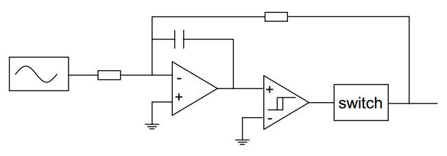
The high frequency oscillation that occurs in a feedback modulator when the feedback signal is too large, is exploited in the self-oscillating class D modulator. See Picture 10. The comparator is equipped with some hysteresis to control the switching frequency. Other factors that influence the switching frequency are the integrator time constant and the output voltage. For large output voltages, the frequency approaches zero. This can cause aliasing problems that can be overcome by using a comparator with a variable hysteresis dependent on the input voltage. In that way the oscillator frequency is kept constant over a wide range of output voltages.


Picture 10: Self oscillating class D modulator


In the situations above, feedback is successfully taken before the output filter. The combination with feedback after the filter is more troublesome.

Output Filter in Class D Amplifier


The output filter is a low pass filter that reduces the switching frequency. When designing the filter, the load impedance is part of the equation. Thus, the load can seriously affect the frequency transfer. For different loudspeakers, the impedance over the audio range can vary from 1 Ω to as much as 30 Ω, with a phase from +56º to - 67º. Picture 1 shows the impedance of a 3-way loudspeaker system that was used in the listening tests.


Picture 1: Loudspeaker impedance


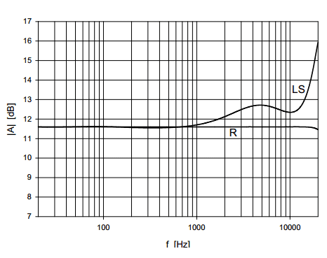
The output filter, however, is designed for a real and constant load impedance. The result of connecting the loudspeaker is shown in Picture 2. The flat line is the simulated transfer of an ideal class D filter followed by a fourth order Butterworth filter with a corner frequency of 30 kHz, loaded with the specified load impedance of 4 Ω. The other line shows what happens when the loudspeaker is connected. The transfer deviates several dB’s from the flat line. This will colour the sound impression. Another problem is that any non-linearities in the filter show up in the distortion figures.


Picture 2: Simulated class D frequency transfer with resistor and loudspeaker load


Feedback can reduce these problems considerably, but because of the phase shift, feedback after (part of) the filter is complicated. In general, the filter (or the filter in combination with lead compensation) must have a first order frequency transfer at 0 dB to ensure stable operation. This is extra complicated by the connected load, which is a part of the filter. High feedback factors can not be realised and feedback around a filter with more than 2-nd order behaviour is very rare. Even when these problems are overcome, the filter prevents further integration because it contains elements that can not be integrated on chip. For sufficient suppression of the carrier frequency, typically a fourth order filter is necessary. In this case, the amount of filtering in practical situations is limited by parasitic capacitances and resistances. Furthermore, two coils and two capacitors are already considered to be many external components. Using only a second order filter is a solution, but the amount of switching ripple can cause EMI problems and the application area of the amplifier will be limited.

Switching Amplifiers - Class D


Linear amplifiers are amplifiers with a linear output stage, in which there exists a voltage drop across the output transistors to generate the correct output voltage. Even though most of these amplifiers use some sort of switching, they are not to be confused with switching amplifiers. Switching amplifiers are amplifiers with a switching output stage. This means that the transistors in the output stage have a switch function. Any simultaneous occurrence of voltage across and current through these transistors is undesirable.


The class D principle


A typical class D amplifier consists of a modulator that converts an analogue or digital audio signal into a high frequency Pulse Width Modulated (PWM) or Pulse Density Modulated (PDM) signal followed by the output stage, often a half bridge power switch (Picture 1). The output of the switches is either high or low, and changes at a frequency that is much higher than the highest audio frequency. Typical values are between 200 kHz and 500 kHz. The frequency spectrum of the PWM signal in the audio band is the same as the frequency spectrum of the audio signal. An LC filter filters out the high frequency switching components, so that the audio signal is available at the output of the filter. Ideally, the switches do not dissipate and neither does the filter, so the efficiency can be very high.


Picture 1: Principle of PWM amplifier


For a 10 kHz sinewave, a switching frequency of 350 kHz, and a filter with a 30 kHz Butterworth characteristic, the signals look like Picture 2. In this case, the audio frequency is close to the corner frequency of the filter, so some phase shift can be observed between the PWM signal and the audio signal.


Picture 2: Class D output signal (before and after the filter)


Output stage


Picture 3 shows a typical class D output stage. It is a class AD stage, which is used for most class D amplifiers. It is a simple inverter. When the input signal is positive, M2 conducts. When it is negative, M1 conducts.


Picture 3: A typical class D output stage


The diodes D1 and D2 are needed because the transistors are unidirectional switches. Suppose the output signal is positive, and the output current Io is also positive. When M1 is switched on, this is OK, but when M2 is switched on, the coil in the output filter still tries to keep the current Io, forcing the output voltage below -VS, causing D2 to conduct. With DMOS transistors as switches, the intrinsic diodes can be used. However, the intrinsic diode of a DMOS transistor can have a long recovery time (several hundred ns) or cause latch-up. In that case external (shottky) diodes are a solution, although not a desirable one. It is also possible to build DMOS transistors with a fast-recovery intrinsic diode.


Switching speed


High switching speeds are necessary to keep switching losses small. Typical values of today’s integrated designs are tens of nanoseconds. Because of the large gate-source capacitances of M1 and M2, this leads to large peak currents. Also, the high speed switching in combination with wires and (gate) capacitances can cause ringing, overshoot, and delays. For a low distortion it is important that the switching times of M1 and M2 are equal. Tuneable coils between M1 and M2 can provide a solution. However, both the fact that these coils can not be integrated and that they need to be tuned make this an unattractive solution. With high speed switching, the risk of common conduction of M1 and M2 increases. The introduction of a "dead zone" in which both transistors are turned off is a common solution, although this introduces extra distortion in the audio signal. Another option is a handshake procedure to check if the other transistor is turned off.


Power supply


In pure feed-forward systems a stable power supply is extremely important, because any deviation from the nominal value shows up in the output signal. For an output signal of 16 bit accuracy, the power supply should have a 16 bit stability. Common solutions are feedback from the pulsed output or feed-forward correction by referring the triangle waveform to the supply voltage. Another supply issue arises from the use of NMOS devices that are preferable thanks to the lower R on per area. The gate of M1 needs a voltage that is higher than VS. A bootstrap capacitor or a charge-pump can provide such a voltage.


Cross-over distortion


M1 and M2 have a certain Ron resistance. D1 and D2 have a certain voltage drop when conducting. Suppose the output current is positive. During conduction of M1, the voltage will be a little lower than VDD because of Ron1. During conduction of D2, the voltage will be a little lower than -VS due to the voltage drop. So all the time the voltage is lower than it should be. When the output current is negative, the same reasoning shows that the output voltage is too high. This results in crossover distortion. It can be solved by connecting the transistors to a tap of the output inductor or a separate supply voltage.


Class BD output stage


An alternative to the class AD stage is the class BD stage. In class BD there are three possible output voltages: positive, negative, and zero. There are several ways in which this can be implemented, but the simplest one is shown in Picture 4.


Picture 4: Class BD modulator with output filter


In quiescent, the signal at A and B is the same PWM signal with 50 % duty cycle. The signal A-B across the filter is therefore zero. For a positive output voltage, the duty cycle of A is increased and that of B decreased. The difference signal A-B is now a voltage that varies between 0 and VS. Similarly, for negative output voltages, A-B varies between 0 and -VS. The pulse frequency of A-B is doubled compared to A and B, which is favourable for speed requirements. Balanced current design has the same qualities and the topologies are very similar. The difference between a bridge class BD stage and a bridge class AD stage is subtle. The topologies are exactly the same. In the class AD case, however, A is always the inverse of B, so that A-B alternates between -VS and VS.


Resonant output stage


A way to generate the high frequency pulses for a PDM modulator is to use a quasi-resonant converter. This converter gives 1 bit each time it is switched on. The bit is not a squarewave, but the positive half of a sinewave. This is irrelevant, as long as the area under the signal is the same each time. For the topology in Picture 5 (Lf and Cf are the output filter) this is true, virtually independent of output current and voltage. Switching occurs when the current is zero, giving better efficiency and lower switching noise. The large number of filter components make this topology not very attractive for use with integrated circuits.


Picture 5: Quasi-resonating converter


Summary and Conclusions


The design of a class D output stage is not a trivial matter. In general, an output stage will not be able to preserve the exact frequency content of its input signal. To summarise the limitations that were encountered, it is easy to start with an important audio amplifier specification: low distortion. With feedback directly from the switched output, very good high power PWM signals can be generated. The output filter, however, introduces additional distortion and deviations of the specified frequency transfer when non-resistive loads are connected. Feedback after the filter is difficult, and high feedback factors can not be realised. Even when these problems are overcome, the filter prevents further integration because for sufficient suppression of the carrier frequency, typically a fourth order filter is necessary. It is not possible to eliminate the external two coils and two capacitors without introducing a much larger switching residue.

Linear amplifiers have a low complexity, can have a low distortion, but show limited possibilities for reduction of the dissipation. To reduce the dissipation to very low values, complex switching schemes are necessary, and a large number of external elcos makes such a solution little attractive. Switching amplifiers can have a very low dissipation, but suffer from switching noise at the output, an external filter, a load dependent frequency transfer and difficulties in achieving a low distortion. The idea that a mix of these two systems may be beneficial is not new, and there are a lot of possibilities for such combinations.