An IEC Variant

The main problem with the IEC signal lies in its need for a noise source. Therefore, a new test signal is proposed that is equivalent to the IEC test signal. The noise source is replaced by 24 square waves of equal amplitude, all a factor 2 in frequency apart. In the frequency range from 10 Hz up to 28 kHz, this simulates pink noise, since the energy per octave is constant. This semi pink noise is filtered to get the IEC frequency characteristics. An additional advantage is that the signal, which had only 24 possible amplitude values, now becomes continuous. Only 100 ms of simulation with this IEC variant suffice, since frequency components below 10 Hz are not present. The square waves are easy to define in a circuit simulator, which will speed up simulations. Also, such a signal can easily be generated in hardware with binary counters or with IC’s that are used as tone generators in electronic organs. To see if this IEC variant is indeed equivalent, the dissipation curves for the three amplifier classes were measured, this time for the IEC signal and its variant. The results in Picture 1 show that the dissipations are almost the same at low output powers. At high output powers, the results differ more. Since heat sink temperature measurements on more than one high power music fragment are not available, it remains unclear if this error is the same for all music fragments at that output power. However, the differences are rather small and only occur when the signal is heavily clipping. At lower, more usual output powers, the IEC variant gives good results.

Picture 1: Measured dissipation of three amplifier classes for the IEC signal and the IEC variant

A Simple Periodic Test Signal

The IEC signal is suitable for measuring the efficiency of audio amplifiers, but for prediction purposes it is less ideal. The signal is difficult to generate when the efficiency of an amplifier has to be simulated in a circuit simulator. In circuit simulators, transient noise sources are rarely available, and usually take a long simulation time. Also, for long term testing (reliability), a noise generator is often not available. A simple, periodic test signal would be welcome. The most important quality is a controlled amplitude probability density function. Suppose the signal is V = f(t), and that it is monotonously rising on t∈ [0,t1]. The distribution function is the chance that f(t) is smaller than a certain value V, is:

Picture 1: The distribution function F(V) and The probability density function f(V)


As it can be seen from Picture 1, the probability density function f(V) is the derivative of the distribution function F(V). So if we want to design a signal with a gaussian amplitude probability density function, we know that f(V) is a gaussian curve. Then, f^-1(V) is the integral of a gaussian curve, which is the normal distribution function. Thus, f(t) must be the inverse of the normal distribution function. Picture 2 shows a possible time function.

Picture 2: Signal with a gaussian amplitude distribution

Picture 3: Frequency distribution of a signal with gaussian amplitude distribution (Picture 2), and of the IEC signal


Unfortunately, the corresponding frequency distribution, shown on Picture 3, is not OK. The higher frequencies are relatively weak. Although the period time of the signal could be chosen a little shorter, the frequency distribution can never match that of the IEC signal. Synthesising a signal that also has a controlled frequency distribution is not straightforward. The signal shown on Picture 2 or a 1/√t signal (which has a 1/f power distribution) can be filtered to produce the signal shown on Picture 4. This signal has a correct frequency distribution, but the amplitude distribution is too wide due to much power in the high amplitudes. Also, the frequency distribution alters when the signal clips, so testing for higher output powers is not possible. When the frequency distribution is of prime importance, the signal of Picture 4 can be useful. However, in practice its application will be very limited.

Picture 4: A signal with an IEC 268 frequency distribution

Conclusion

It seems hardly possible to construct a simple periodic test signal that has all the properties we need to simulate music and speech. Often, however, the amplitude distribution is the most important property. Class G amplifiers, for instance, are not very sensitive to the exact frequency of their output signal. In that case, the signal of Picture 2 is advantageous owing to its very short repetition frequency. In a circuit simulator, a single period will suffice to give a good dissipation prediction.

Measuring and Estimating Amplifier Power Dissipation

It is important that the efficiency of audio amplifiers is measured correctly. Good test signals and adequate measurement procedures are crucial to make fair comparisons between amplifiers and reliably predict the dissipation in practical situations. This is also a vital condition for judging the usefulness of new amplifier topologies.

In literature, the efficiency of amplifiers is usually measured with sinusoidal signals. For amplifiers based on a class D topology, this gives approximately the same results as for audio signals, as long as one bears in mind that the average output power of an audio amplifier while playing normal audio signals is much lower than its maximum sine output power. Some high efficiency audio amplifiers, however, need specific audio characteristics to obtain a high efficiency. Well known topologies in this field are the class G and class H principles. The amplifiers which use knowledge about either the amplitude or the frequency distribution of average audio signals, measurements with sinusoids can give pessimistic results.

The best signal would be a real audio signal, but this has several disadvantages. The question is which audio signal should be taken. Speech? Music? What kind of music? This is not standardised. Furthermore, at least several seconds of audio are necessary to get a good impression, which is not very practical for simulations. Also, a music signal does not give stable readings on meters. In practice, more creative ways were found. Either the efficiency was measured indirectly by measuring heat sink temperatures, or an ad hoc measure is defined. Another possibility is to use the IEC-268 "simulated programme material". The spectral distributions of programme material were measured, and the latter also investigated whether the IEC test signal is useful for evaluating the power rating of loudspeakers. There is, however, no standard test signal intended for measuring or predicting amplifier efficiency. However, we can try to find such a signal. For that reason, please refer to the articles Characteristics of Audio Signals and The IEC-268 Test Signal.

Completeness

Despite the good characteristics of the IEC signal, one can still wonder if these characteristics are complete, do they fully determine amplifier dissipation? To answer this, three amplifiers were built: a standard class AB amplifier, a class H amplifier (an amplifier that lifts the power supply during signal peaks by means of an electrolytic capacitor), and a class D + AB amplifier (an amplifier that has a class AB and a class D amplifier in parallel). The class AB amplifier is only sensitive to the amplitude distribution of its output signal, the frequency is not important. The class H amplifier dissipation is "to some extent" frequency dependent, because charging and discharging the capacitor is not lossless, so the total dissipation of this amplifier depends on both the volume and the frequency of the output signal. Finally, the class D + AB amplifier is also sensitive to both characteristics. The class AB part in this amplifier has to support the output current for high d(Iout)/dt, starting at 1 kHz full scale signal swing. All amplifiers have a maximum output power of 30 W, and have identical heat sinks.

Input to the amplifiers are both the IEC signal and a music fragment that is selected because it has almost identical characteristics (a fragment of "Me and Bobby McGee" by Janis Joplin). Measured are the heat sink temperatures as a function of time of all amplifiers. The results are depicted in Picture 1. The average output power was 2 W, at which the amplifiers were clipping a negligible part of the time. The difference in dissipation between the two signals is insignificant. When the average output power is increased to 10 W, the music and the test signal are clipping a considerable part of the time. Even then, there is hardly any difference between the two, as is shown in Picture 2. The differences that do occur can be explained by measurement inaccuracies or slight differences between the amplitude distributions.

Picture 1: Heat sink temperatures for three amplifier classes and two signals at an average output power of 2 W (no clipping)

Picture 2: Heat sink temperatures for three amplifier classes and two signals at an average output power of 10 W (heavy clipping)


With these results it seems that the amplitude and frequency characteristics fully determine amplifier dissipation, also under clipping conditions. Thus we can trust that the dissipation of audio fragments with the same characteristics as the IEC signal will also cause the same dissipation.

Accuracy

Although the IEC characteristics are a good average, individual fragments can have characteristics that are quite different. The question arises if these fragments produce amplifier dissipations that are also significantly different. To answer this question, it is necessary to measure the dissipation of the three amplifier classes for all audio fragments. Direct measurement of amplifier efficiency for audio signals, however, is difficult. One possibility is measuring the heat sink temperature, as was done in the previous section. This requires a constant ambient temperature and is very time consuming. Another (complicated) possibility is sampling the output voltage and the supply current, and calculate the dissipation. To circumvent these drawbacks, behavioural models of the amplifiers are used, and the dissipation is simulated with C programs, evaluating the dissipated energy per audio sample. With the proper models, it is easy to calculate the dissipations for the various audio fragments. The models were developed with the IEC signal measurement results as reference. To demonstrate the validity for real audio signals, Picture 3 shows the simulated dissipation for both the IEC signal and the fragment of Janis Joplin. The dissipations are practically the same, as they should be. Furthermore, the ratios between amplifier dissipations at 2 W and 10 W deviate less than 15 % from the ratios of the extrapolated increase in heat sink temperatures of Picture 1 and Picture 2.

Picture 3: Simulated dissipation of three amplifier classes (for the IEC test signal and a fragment of Janis Joplin)


After all audio fragments were scaled to equal power, the dissipation they caused was calculated for all amplifier classes. Picture 4 shows the results as a histogram. It has a logarithmic x-axis. The distance between the left border and the right border of each bar is a factor 1.05. The height of the bar indicates how many audio fragments cause a dissipation in that range. The vertical lines indicate the dissipation for the IEC signal. It appears that all fragments have dissipations within +/- 20 % of the dissipation predicted by the IEC test signal. One fragment stands out because it causes a high dissipation in both the class D + AB and the class H amplifier. The large high frequency contents decreases the efficiency of the two amplifiers. Although this is an exceptional case, it is important to realise that the good predictive qualities of the IEC signal might not be valid for an amplifier which is more sensitive to the frequency contents of its input signal. In general, however, the IEC signal is representative for a wide range of audio signals.

Picture 4: Histogram of the simulated dissipation of all audio fragments in 3 amplifier classes (Vertical lines indicate the dissipation for the IEC signal)

Conclusions

For the tested types of high-efficiency amplifiers: a class AB, a class H, and a class D + AB amplifier. The power, the amplitude distribution and the frequency distribution of the output signal fully determine the amplifier’s dissipation. The Peak-to-Average ratio of the signal is not very significant.
The dissipation for a variety of real-life audio signals of constant volume deviates only 20 % from the dissipation caused by the IEC 268 test signal at the same output power. Therefore, this signal is very suitable for measuring audio amplifier efficiency. This must be verified for new amplifiers types, that may be more sensitive to amplitude or frequency distribution deviations.
Two alternative test signals are proposed. For simulation and test purposes, a simple test signal can be used for amplifiers with near frequency independent dissipation (A Simple Periodic Test Signal). When the frequency contents is also important, an IEC look-alike test signal can be used which has the same characteristics as the IEC signal (An IEC Variant), but is easier to generate in simulation and hardware.

The IEC-268 Test Signal

The International Electrotechnical Commission (IEC) has defined a noise input signal representative for normal programme material. It is generated by a pink or white noise source followed by a filter. We will refer to this signal as the "IEC signal", and investigate if it is useful for efficiency measurements (more of this in next articles).

Characteristics

Picture 1 shows that the amplitude distribution of the IEC signal is gaussian.

Picture 1: Amplitude distribution of the IEC-268 test signal and a gaussian curve as reference


Picture 2 shows the IEC signal frequency distribution, together with the distribution of the fragments (discussed in Characteristics of Audio Signals). The IEC signal serves well as a typical audio fragment.

Picture 2: Frequency distribution of the fragments and of the IEC test signal (fat line)

Characteristics of Audio Signals

The test set

In order to compare test signals to realistic audio signals, it is necessary to define a test set of audio fragments. Due to the variation in volume in audio signals, the statistical parameters depend on the length of the time interval that is being analysed. Picture 1 shows the amplitude distribution of complete CD tracks. Compared to shorter fragments with constant volume (see Picture 2), we notice a somewhat larger spread and a clearly different shape which peaks around zero amplitude. This is a result of the sections with a lower volume. Now suppose we would use the distributions of Picture 1 to predict amplifier dissipation. Such a signal has a certain average power that has to be delivered by the amplifier, leading to a certain (predicted) average dissipation. During the loud passages, however, the amplifier has to deliver considerably more power, and when they last longer than the heat sink’s thermal time constant, the amplifier will overheat. Therefore, we have chosen audio fragments with constant volume. Of course it should be noted that "constant" is a relative measure, since the audio waveform itself is not constant. It is assumed that variations in less than seconds will not give rise to the problems described above.
There are chosen 80 fragments from various CD’s, including classical music, pop music, jazz, hard rock, house, heavily compressed music, and speech signals. The length of each fragment is between 3 and 12 s. The volume during each fragment is constant. All fragments were converted to mono and normalised to full scale, with the highest sample just clipping. The number of bits per sample was reduced to 8 to get smoother amplitude distributions. Because the fragments are normalised to full scale, this barely affects the sound impression.

Picture 1: Amplitude distributions (of 36 CD tracks, normalised to 1 at zero amplitude and then scaled to equal power)

Amplitude distribution

The amplitude distribution is determined by counting how many samples with a certain amplitude (28 = 256 levels) occur in one fragment. Picture 2 shows the amplitude distribution of all 80 fragments.

Picture 2: Amplitude distributions (of all fragments, normalised to 1 at zero amplitude and then scaled to equal power)


It confirms that the shape of the amplitude distribution is gaussian. There are a few exceptions, though. Firstly, one curve has two peaks symmetrically around zero amplitude. This is the distribution of a fragment hard-core house music, that contains purely synthesised sounds. Although this is an exceptional case, it shows the importance of realising that certain audio characteristics can differ significantly from the average case. Secondly, we see some very narrow curves. These are the distributions of speech signals. Due to the pauses inherent to spoken word, the distributions peak around zero amplitude.
When discussing amplitude distributions, it is useful to critically examine the Peak-to-Average Ratio (PAR). It is widely acknowledged as a signal property, and identical to the traditional crest factor. Expressed in dB’s, the PAR is defined as:

PAR = 20*log(U(t)max/URMS)


Picture 3 shows the PAR-s of all fragments. Roughly, it is between 10 dB and 20 dB, with an average of 15 dB. This means that "in order to be undistorted" the average audio fragment must have a power at least 12 dB below a full power sinewave.

Picture 3: Peak-to-Average ratios (of all fragments)


Often, the PAR is also used for calculating amplifier efficiencies, resulting in a certain efficiency for a certain PAR of the signal. In that case it is assumed that every fragment is amplified to a level just below clipping. The result is that the amplifier dissipation strongly depends on the PAR. The reason for this is, that the average power (or URMS) also varies considerably, since U(t)max is the clipping point of the amplifier and therefore constant. In Picture 2, however, it can be seen that, when scaled to equal power, the amplitude distributions are almost the same. U(t)max varies, but since the high amplitudes near U(t)max are unlikely to occur, they hardly effect the total dissipation of the amplifier. When a fragment with a large PAR is amplified to equal power as a fragment with a low PAR, there will be some clipping, but this is barely perceptible in normal listening conditions. Only when we increase the volume a lot, the sound quality degrades. Subjective listening tests show that the PAR can be made as small as 6dB before most fragments sound really bad through clipping. A PAR of 6dB means that the output power is half the maximum sine power. From the above we conclude the following: Audio fragments of constant volume generally have a gaussian amplitude distribution with an average PAR of 15dB. Concerning amplifier dissipation, average power is the most important variable, while the PAR does not play a significant role. Amplifier dissipation for gaussian signals must be tested up to half the full sine power.

Frequency distribution

On the same audio fragments, a Fast Fourier Transform (FFT) was performed over the full length. A normal log-log bode plot of the frequency content (Picture 4) does not provide very useful information.

Picture 4: Traditional graph of a Fourier transform of a music fragment (Vertical scale dB’s are relative to full scale for measurement bandwidth 2/Tfragment)


Firstly, there is no need for a high accuracy, so it seems more logical to choose the vertical scale of the plot linear instead of logarithmic. Secondly, efficiency is a matter of power. When an amplifier has a better efficiency for certain frequencies, it is important to know how much power is present in those frequencies, not how much amplitude. So it’s more useful to square the amplitudes. Finally, the squared FFT gives the power of the frequencies in the signal. The frequencies are linearly spaced. With a logarithmic frequency axis, a temptation exists to overemphasise the lower frequencies because they are relatively enlarged. A linear frequency axis might seem a logical choice, but since pitch perception is logarithmic in nature (every octave higher equals a factor two), it is preferable to use a logarithmic axis, and plot the sum of the squared Fourier coefficients. An extra advantage is that the summation smoothens the curve.
Presented in this way, the frequency distribution is a line that starts at (almost) power = 0 at 20 Hz, climbing to power = 1 at 20 kHz. The frequency distributions of all fragments are shown on Picture 5. The average fragment is S-shaped, with a mid-frequency part corresponding to a straight line between (50 Hz, 0) and (3 kHz, 1). This does not come as a surprise when we realise that the notes in a musical scale are fixed factors in frequency apart, in which case a linear frequency distribution requires all notes to be equally loud. In Picture 5, the fragments with much power in the lower frequencies have a house beat or a contrabass. The fragments with much power in the higher frequencies mostly have electric guitars or synthesisers. One fragment in particular stands out because it contains much more high frequencies than the others. It is the intro of Melissa Etheridge’s "Like the way I do", containing a guitar and a tambourine.

Picture 5: Frequency distribution (of all audio fragments)

Additional Specifications of Power Amplifiers

The list of additional specifications of power amplifiers can be endless. However, we will mention here some of them which are more important.

Damping Factor

A flat frequency response is desirable to avoid tonal coloration, but a flat response may not always be obtained when the amplifier is driving a real-world loudspeaker load. The input impedance of real loudspeakers can vary dramatically as a function of frequency, while the output impedance of the power amplifier is nonzero. A voltage divider is thus formed by the amplifier output impedance and the loudspeaker input impedance. Here the amplifier is modeled with an ideal amplifier with zero output impedance in series with impedance Zout that describes its actual output impedance (referred to as a Thévénin equivalent circuit). This is where the damping factor (DF) comes into play. In spite of its important-sounding name, this is just a different way of expressing the output impedance of the amplifier.
While amplifiers ideally act like voltage sources with zero output impedance, they all have finite output impedance. The term damping factor came from the fact that a loudspeaker is a mechanically resonant system; the low output impedance of an amplifier damps that resonance via the resistance of the loudspeaker’s voice coil and electromotive force. An amplifier with higher output impedance will provide less damping of the loudspeaker cone motion because it adds to the total amount of resistance in the circuit. Damping factor is defined as the ratio of 8 Ω to the actual output impedance of the amplifier. Thus, an amplifier with an output impedance of 0.2 Ω will have a DF of 40.
Most vacuum tube amplifiers have a DF of less than 20, while many solid-state amplifiers have a DF in excess of 100. It is important to bear in mind that the DF is usually a function of frequency, often being larger at low frequencies. This is consistent with the need to dampen the cone motion of woofers, but ignores the influence of the DF on frequency response at higher frequencies. Many loudspeakers have a substantial peak or dip in their impedance at or near their crossover frequencies. This could result in coloration if the amplifier DF is low.
The effect of damping factor and output impedance on frequency response must not be underestimated in light of the large impedance variations seen in many contemporary loudspeakers. It is not unusual for a loudspeaker’s impedance to dip as low as 3 Ω and rise as high as 40 Ω across the audio band. Consider this wildly varying load against the 0.4 Ω output impedance of a vacuum tube amplifier with a DF of 20. This will cause an audible peak-to-peak frequency response variation of ± 0.5 dB across the audio band.

Dynamic Headroom

Unlike a sine wave, music is impulsive and dynamic. Its power peaks are often many times its average power. This ratio is often referred to as the crest factor. Dynamic headroom refers to the fact that an amplifier can usually put out a greater short-term burst of power than it can on a continuous basis. The primary cause of this is power supply sag which is a reflection of power supply regulation. The power supply voltages will initially remain high and near their no-load values for a brief period of time during heavy loading due to the energy storage of the large reservoir capacitors. Under long-term conditions, the voltage will sag and less maximum power will be available. Consider an amplifier that clips at 100 W into 8 Ω on a continuous test basis. If this amplifier has a power supply with 10% regulation from no-load to full load (which is fairly good), the available power supply voltage will be about 10% higher during a short-term burst. This will result in a short-term power capability on the order of 120 W, since power goes as the square of voltage.
Dynamic headroom is a two-edged sword. It is good to have it because music tends to have an average power level much lower than the brief peak power levels it can demand (referring again to the crest factor). It is nice to have 20% to 40% more power available when it is needed for those brief peaks. On the other hand, a large amount of dynamic headroom is often symptomatic of an amplifier with a sloppy power supply.

Slew Rate

Slew rate is a measure of how fast the output voltage of the amplifier can change under large-signal conditions. It is specified in volts per microsecond. Slew rate is an indicator of how well an amplifier can respond to high-level transient program content. A less capable amplifier might have a slew rate of 5 V/µs, whereas a really high-performance amplifier might have a slew rate on the order of 50 to 300 V/µs. For a given type of program material, a higher-power amplifier needs to have a higher slew rate to do as well as a lower-power amplifier, since its voltage swings will be larger. A 100-W amplifier driving a loudspeaker whose efficiency is 85 dB will need to have 3.16 times the amount of slew rate capability as a 10-W amplifier driving a 95 dB speaker to the same sound pressure level.
As a point of reference, the maximum voltage rate of change of a 20 kHz sine wave is 0.125 V/µs per volt peak. This means that a 100-W amplifier that produces a level of 40 V peak at 20 kHz must have a slew rate of at least 5 V/µs. In practice a much larger value is desirable for low-distortion performance on high-frequency program content. Although technically imprecise, the rate of change of a signal is often referred to its slew rate for convenience.
The slew rate capability of audio power amplifiers received a lot more attention after the term transient inter-modulation distortion (TIM) was coined and studied intensely during the 1970s and early 1980s. This was largely another way of describing high-frequency distortion that resulted from slew rate deficiency.

Output Voltage and Current

Here we will briefly touch on the reality of output voltage and current swing that an amplifier may have to deliver in practice. The first table on Picture 1 shows the RMS value of the sine wave voltage, the peak voltage, the peak current, and the reserve current required for the popular 8 Ω resistive load as a function of power. The reserve current listed below is simply a factor of three greater than the peak current required of a resistive load and represents the reality of driving difficult reactive loudspeaker loads with non-sinusoidal wave forms. The reserve current can be assumed to occur only in a brief time interval under fairly rare circumstances.

Picture 1: Voltage and Current into a 8, 4 and 2 Ω Load


This data gives a glimpse of what is necessary for the amplifier to provide. Notice the very substantial voltage swings, and implied power supply voltages, required for a 400 W amplifier. The peak and reserve currents are also into the tens of amperes at 400 W. This is just the beginning of the story, however. The second table shows what the same amplifier would encounter when driving a 4 Ω load. Here we have assumed that the drive signal has remained the same and only the load impedance has dropped. We have also implicitly assumed that the amplifier has ideal power supply regulation, so all of the power numbers are doubled.
Given the nature of some of today’s high-end loudspeakers, some have argued that really high-performance amplifiers should be rated for power delivery into 2 Ω (at least for short intervals). Indeed, the testing done in some amplifier technical reviews regularly subjects power amplifiers to a 2 Ω resistive load test. The figures for output current become almost bewildering under these conditions. An important point here is that there are amplifiers sold every day that are rated at up to 400 W per channel into 8 Ω, and designers implement such amplifiers every day.
The sobering point is that if at the same time the designer thinks in terms of his amplifier being 2 Ω compatible, the potential demanded burst current could on occasion be quite enormous. This is illustrated in third table shown on Picture 1.

Basic Specifications of Power Amplifiers

Essentially, an audio amplifier is a normal voltage amplifier optimised for the amplification of audio signals. The limited frequency response of the ear sets the bandwidth limits: 20 Hz - 20 kHz, although most people are not able to hear 20kHz. Most power is concentrated in the mid frequencies, and occasionally in the low frequencies. Generally, the amplitude probability density function of audio signals is gaussian. This means that the ratio between maximum and average power is large: 10 … 20 dB. In average, it is 15 dB, which is 12dB below the power of a rail-to-rail sinewave. The primary specifications of an audio power amplifier include maximum power, frequency response, noise, and distortion.

Rated Output Power

The ear has a very large dynamic range. To give an example: the ratio between the acoustic power of a rock concert and the sound of breathing can be as large as 10^11. This makes large demands on the dynamic range of the audio amplifier.
Maximum output power is almost always quoted for a load of 8 Ω and is often quoted for a load of 4 Ω as well. A given voltage applied to a 4 Ω load will cause twice the amount of current to flow, and hence twice the amount of power to be delivered. Ideally, the output voltage of the power amplifier is independent of the load, both for small signals and large signals. This implies that the maximum power into a 4 Ω load would be twice that into an 8 Ω load. In practice, this is seldom the case, due to power supply sag and limitations on maximum available output current.
The correct terminology for power rating is continuous average sine wave power, as in 100 W continuous average sine wave power. However, many often take the liberty of using the term W RMS. Although technically incorrect, this wording simply is referring to the fact that the power would have been measured by employing a sine wave whose RMS AC voltage was measured on a long-term basis. There are other ways of rating power that are sometimes used because they provide larger numbers for the marketing folks, but we will ignore them here. When you hear terms like peak power just realize that these are not the same as the more rigorous continuous average power rating.

Frequency Response

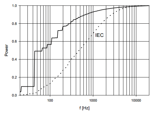
The frequency response of a power amplifier must extend over the full audio band from 20 Hz to 20 kHz within a reasonable tolerance. Modern amplifiers usually far exceed this range, with frequency response from 5 Hz to 200 kHz not the least bit uncommon. The frequency response for such an amplifier is illustrated with the solid curve on Picture 1. While the tolerance assigned to the frequency response of loudspeakers is often ± 3 dB, the tolerance associated with power amplifiers is usually + 0 dB, – 3 dB, or tighter. Specifying where an amplifier is down by 3 dB from the nominal 0 dB reference is the conventional way of specifying the bandwidth of a system. This is often referred to as the 3-dB bandwidth. The frequency response for a less capable amplifier is shown with the dashed curve on Picture 1. This amplifier has a 3-dB bandwidth from 10 Hz to 80 kHz. Its response is down 1 dB at 20 Hz and 0.5 dB at 20 kHz.

Picture 1: Amplifier frequency response

Noise

It is important that power amplifiers produce low noise, since the noise they make is always there, independent of the volume control setting and the listening level. This is particularly so when the amplifiers are used with high-efficiency loudspeakers. The noise is usually specified as being so many decibels down from either the maximum output power or with respect to 1 W. The former number will be larger by 20 dB for a 100 W amplifier, so it is often the one that manufacturers like to cite. The noise referenced to 1 W into 8 Ω (or, equivalently, 2.83 V RMS) is the one more often measured by reviewers.
The noise specification may be unweighted or weighted. Unweighted noise for an audio power amplifier will typically be specified over a full 20-kHz bandwidth (or more). Weighted noise specifications take into account the ear’s sensitivity to noise in different parts of the frequency spectrum. The most common one used is A weighting, illustrated on Picture 2. Notice that the weighting curve is up about +1.2 dB at 2 kHz and down 3 dB at approximately 500 Hz and 10 kHz.

Picture 2: A weighting frequency response


The A-weighted noise specification for an amplifier will usually be quite a bit better than the unweighted noise because the weighted measurement tends to attenuate noise contributions at higher frequencies and hum contributions at lower frequencies. A very good amplifier might have an unweighted signal to noise ratio (S/N) of 90 dB with respect to a 1-W output into 8 Ω, while that same amplifier might have an A-weighted S/N of 105 dB with respect to 1 W. A fair amplifier might sport 65 dB and 80 dB S/N figures, respectively. The A-weighted number will usually be 10–20 dB better than the unweighted number.

Distortion

The most common distortion specification is total harmonic distortion (THD). It will usually be specified at one or two frequencies or over a range of frequencies. It will be typically specified at a given power level with the amplifier driving a specified load impedance. A good 100-W amplifier might have a 1 kHz THD (referred to as THD-1) of 0.005% at 100 W into 8 Ω. That same amplifier might have a 20-kHz THD (THD-20) of 0.02% up to 100 W into 8 Ω. Although 1 kHz THD is at a frequency in the middle of the audible frequency range where hearing sensitivity is high, it is not very difficult to achieve low THD figures at 1 kHz. Good THD-20 performance is much more difficult to achieve and is generally a better indicator of amplifier performance.
In practice, the harmonic distortion specification will be described as THD + N, where the N refers to noise. This reflects the way in which THD is most often measured. When measuring THD-1, a 1 kHz fundamental sine wave is applied to the amplifier input. The 1 kHz fundamental appearing in the output signal is then notched out by a very sharp filter. Everything else, both distortion harmonics and noise, is measured, giving rise to the THD + N specification. At higher power testing levels, the true THD will often dominate the noise, but at lower power levels the measurement may often reflect the noise rather than the actual THD being measured. Graphs that show rising THD + N at lower power levels can be misleading. The rising level may actually be noise rather than distortion. This is because a fixed noise voltage becomes a larger percentage of the level of the fundamental as the fundamental decreases in amplitude at lower power levels.
The Federal Trade Commission (FTC) long ago tried to wrap things up in a single statement that would largely capture power, distortion, and bandwidth together. It would read something like “100-W continuous average power from 20 Hz to 20 kHz with less than 0.02% total harmonic distortion.” This was a reasonably comprehensive and honest way to describe the most basic capability of an amplifier. It is unfortunate that it has fallen into disuse by many manufacturers. Part of the reason was that it also required that the amplifier could be run at 1/3 rated power into 8 Ω for an extended period of time without overheating. Operating at 1/3 rated power is close to the point where most amplifiers dissipate the most heat, and it was expensive for many amplifier manufacturers to provide enough heat sinking to meet this requirement.

Total Harmonic Distortion (THD)

When a sinusoidal signal is applied to a non-linear amplifier, the output contains the base frequency plus higher order components that are multiples of the base frequency. The Total Harmonic Distortion is the ratio between the power in the harmonics and the power in the base frequency. This can be measured on a spectrum analyser. Most distortion analysers, however, subtract the base signal from the amplifier’s output and calculate the ratio between the total RMS value of the remainder and the base signal. This is called THD+N: Total Harmonic Distortion + Noise. Normally, the noise will be low compared to the distortion, but the noise of a noisy amplifier or the switching residues in a class D amplifier can give garbled THD figures. For a THD+N measurement, the bandwidth must be specified. For class D measurements, a sharp filter with a 20kHz corner frequency is necessary to prevent switching residues - that are inaudible - to show up in the distortion measurements.

InterModulation distortion (IM)

When two sinusoids are summed and applied to a non-linear amplifier, the output contains the base frequencies, multiples of the base frequencies and the difference of (multiples of) the base frequencies. Suppose a 15 kHz sinusoid is applied to an audio system that has a 20 kHz bandwidth, and the THD+N needs to be measured. All the harmonics are outside the bandwidth and will be attenuated, resulting in too low a THD+N reading. The same situation occurs when the distortion analyser has a 20 kHz bandwidth. In these cases, an IM measurement can be a solution.
The first standard was defined by the SMPTE (Society of Motion Picture and Television Engineers). A 60Hz tone and a 7kHz tone in a 4:1 amplitude ratio are applied to the non-linear amplifier. The 60Hz appears as sidebands of the 7kHz tone. The intermodulation distortion is the ratio between the power in the sidebands and the high frequency tone. Another common standard is defined by the CCITT (Comité Consultatif Internationale de Télégraphie et Téléphonie), and uses two tones of equal strength at 14kHz and 15kHz. This generates low frequency products and products around the two input frequencies, depending on the type (odd or even) of distortion.

Interface InterModulation distortion (IIM)

In this test, the second tone of an IM measurement set-up is not connected to the input, but to the output (in series with the load impedance).

Transient InterModulation distortion (TIM)

When a squarewave is applied to an amplifier with feedback, its input stage has to handle a large difference signal, probably pushing it into a region that is less linear than its quiescent point. When a sinusoid is added to the squarewave, the nonlinearity induced by the edges of the squarewave will distort the sinusoid, giving rise to TIM, also called transient distortion or slope distortion. There are many ways of testing TIM and it remains unclear how much it adds to the existing measurement methods. If the maximum input signal frequency during normal operation of an amplifier is limited to 20 kHz, a 20 kHz full power sinusoid is the worst case situation. When that generates little distortion, TIM will not occur.

Cross-over distortion

Cross-over distortion is generated at the moment the output current changes sign. At that moment, the output current gets supplied by another output transistor. The process of taking over generates distortion, visible as spikes in the residual signal of a THD measurement. This kind of distortion is notorious for its unpleasant sound (a small percentage error is quickly noticeable). Because it’s usually present around zero amplitude, the impact on small signals can be relatively large.