Controller Algorithms and Tuning


In the previous articles of this category were described the purpose of control, defined individual elements within control loops, and demonstrated the symbology used to represent those elements in an engineering drawing. The examples of control loops used thus far have been very basic. In practice, control loops can be fairly complex. The strategies used to hold a process at setpoint are not always simple, and the interaction of numerous setpoints in an overall process control plan can be subtle and complex. In this article, you will be introduced to some of the strategies and methods used in complex process control loops. The goal of this article is to:

❑ Differentiate between discrete, multistep, and continuous controllers.
❑ Describe the general goal of controller tuning.
❑ Describe the basic mechanism, advantages and disadvantages of the following mode of controller action:
• Proportional action;
• Intergral action;
• Derivative action;
❑ Give examples of typical applications or situations in which each mode of controller action would be used.
❑ Identify the basic implementation of P, PI and PID control in the following types of loops:
• Pressure loop;
• Flow loop;
• Level loop;
• Temperature loop.


Controller Algorithms


The actions of controllers can be divided into groups based upon the functions of their control mechanism. Each type of controller has advantages and disadvantages and will meet the needs of different applications. Grouped by control mechanism function, the three types of controllers are:

❑ Discrete controllers
❑ Multistep controllers
❑ Continuous controllers


Discrete controllers


Discrete controllers are controllers that have only two modes or positions: on and off. A common example of a discrete controller is a home hot water heater. When the temperature of the water in the tank falls below setpoint, the burner turns on. When the water in the tank reaches setpoint, the burner turns off. Because the water starts cooling again when the burner turns off, it is only a matter of time before the cycle begins again. This type of control doesn’t actually hold the variable at setpoint, but keeps the variable within proximity of setpoint in what is known as a dead zone (Picture 1).


Picture 1: Discrete Control


Multistep controllers


Multistep controllers are controllers that have at least one other possible position in addition to on and off. Multistep controllers operate similarly to discrete controllers, but as setpoint is approached, the multistep controller takes intermediate steps. Therefore, the oscillation around setpoint can be less dramatic when multistep controllers are employed than when discrete controllers are used (Picture 2).


Picture 2: Multistep Control Profile


Continuous controllers


Controllers automatically compare the value of the PV to the SP to determine if an error exists. If there is an error, the controller adjusts its output according to the parameters that have been set in the controller.


Picture 3: Automatic Feedback Control


The tuning parameters essentially determine (Picture 3):

>> How much correction should be made? The magnitude of the correction (change in controller output) is determined by the proportional mode of the controller.
>> How long should the correction be applied? The duration of the adjustment to the controller output is determined by the integral mode of the controller.
>> How fast should the correction be applied? The speed at which a correction is made is determined by the derivative mode of the controller.

Mode of Operation of different Controller Types


This article explains the control response of various controller types and the significance of parameters. As in the explanation of controlled systems, the step response is used for this description. The input variable to the controller is the system deviation – that is, the difference between the desired value and the actual value of the controlled variable.


Proportional (P) controller


In the case of the proportional controller, the actuation signal is proportional to the system deviation. If the system deviation is large, the value of the manipulated variable is large. If the system deviation is small, the value of the manipulated variable is small. The time response of the P controller in the ideal state is exactly the same as the input variable (see Picture 1).


Picture 1: Time response of the P controller


The relationship of the manipulated variable to the system deviation is the proportional coefficient or the proportional gain. These are designated by xp, Kp or similar. These values can be set on a P controller. It determines how the manipulated variable is calculated from the system deviation. The proportional gain is calculated as:

Kp = y0 / x0


If the proportional gain is too high, the controller will undertake large changes of the manipulating element for slight deviations of the controlled variable. If the proportional gain is too small, the response of the controller will be too weak resulting in unsatisfactory control. A step in the system deviation will also result in a step in the output variable. The size of this step is dependent on the proportional gain. In practice, controllers often have a delay time, that is a change in the manipulated variable is not undertaken until a certain time has elapsed after a change in the system deviation. On electrical controllers, this delay time can normally be set. An important property of the P controller is that as a result of the rigid relationship between system deviation and manipulated variable, some system deviation always remains. The P controller cannot compensate this remaining system deviation.


Integral-action (I) controller


The I controller adds the system deviation over time. It integrates the system deviation. As a result, the rate of change (and not the value) of the manipulated variable is proportional to the system deviation. This is demonstrated by the step response of the I controller: if the system deviation suddenly increases, the manipulated variable increases continuously. The greater the system deviation, the steeper the increase in the manipulated variable (see Picture 2).


Picture 2: Time response of the I controller


For this reason the I controller is not suitable for totally compensating remaining system deviation. If the system deviation is large, the manipulated variable changes quickly. As a result, the system deviation becomes smaller and the manipulated variable changes more slowly until equilibrium is reached.
Nonetheless, a pure I controller is unsuitable for most controlled systems, as it either causes oscillation of the closed loop or it responds too slowly to system deviation in systems with a long time response. In practice there are hardly any pure I controllers.


PI controller


The PI controller combines the behaviour of the I controller and P controller. This allows the advantages of both controller types to be combined: fast reaction and compensation of remaining system deviation. For this reason, the PI controller can be used for a large number of controlled systems. In addition to proportional gain, the PI controller has a further characteristic value that indicates the behaviour of the I component: the reset time (integral-action time).


Picture 3: Time response of the PI Controller


Reset time


The reset time is a measure for how fast the controller resets the manipulated variable (in addition to the manipulated variable generated by
the P component) to compensate for a remaining system deviation. In other words: the reset time is the period by which the PI controller is faster than the pure I controller. Behaviour is shown by the time response curve of the PI controller (see Picture 3).

The reset time is a function of proportional gain Kp as the rate of change of the manipulated variable is faster for a greater gain. In the case of a long reset time, the effect of the integral component is small as the summation of the system deviation is slow. The effect of the integral component is large if the reset time is short. The effectiveness of the PI controller increases with increase in gain Kp and increase in the I-component (i.e., decrease in reset time). However, if these two values are too extreme, the controller’s intervention is too coarse and the entire control loop starts to oscillate. Response is then not stable. The point at which the oscillation begins is different for every controlled system and must be determined during commissioning.


PD controller


The PD controller consists of a combination of proportional action and differential action. The differential action describes the rate of change of the system deviation. The greater this rate of change – that is the size of the system deviation over a certain period – the greater the differential component. In addition to the control response of the pure P controller, large system deviations are met with very short but large responses. This is expressed by the derivative-action time (rate time).


Picture 4: Time response of the PD Controller


Derivative-action time


The derivative-action time Td is a measure for how much faster a PD controller compensates a change in the controlled variable than a pure P controller. A jump in the manipulated variable compensates a large part of the system deviation before a pure P controller would have reached this value. The P component therefore appears to respond earlier by a period equal to the rate time (see Picture 4).

Two disadvantages result in the PD controller seldom being used. Firstly, it cannot completely compensate remaining system deviations. Secondly, a slightly excessive D component leads quickly to instability of the control loop. The controlled system then tends to oscillate.


PID controller


In addition to the properties of the PI controller, the PID controller is complemented by the D component. This takes the rate of change of the system deviation into account. If the system deviation is large, the D component ensures a momentary extremely high change in the manipulated variable. While the influence of the D component falls of immediately, the influence of the I component increases slowly. If the change in system deviation is slight, the behaviour of the D component is negligible. This behaviour has the advantage of faster response and quicker compensation of system deviation in the event of changes or disturbance variables. The disadvantage is that the control loop is much more prone to oscillation and that setting is therefore more difficult. Picture 5 shows the time response of a PID controller.


Picture 5: Time response of the PID Controller


Derivative-action time


As a result of the D component, this controller type is faster than a P controller or a PI controller. This manifests itself in the derivative-action time Td. The derivative-action time is the period by which a PID controller is faster than the PI controller.


Controllers


The previous article Controlled System, dealt with the controlled system - the part of the system which is controlled by a controller. This article is about the controller. The controller is the device in a closed-loop control that compares the measured value (actual value) with the desired value, and then calculates and outputs the manipulated variable. The above section showed that controlled systems can have very different responses. There are systems which respond quickly, systems that respond very slowly and systems with storage property.
For each of these controlled systems, changes to the manipulated variable y must take place in a different way. For this reason there are various types of controller each with its own control response. The control engineer has the task of selecting the controller with the most suitable control response for the controlled system.


Control response


Control response is the way in which the controller derives the manipulated variable from the system deviation. There are two broad categories: continuous-action controllers and non-continuous-action controllers.


Continuous-action controller


The manipulated variable of the continuous-action controller changes continuously dependent on the system deviation. Controllers of this type give the value of the system deviation as a direct actuating signal to the manipulating element. An example of this type of controller is the centrifugal governor (Picture 1). It changes its moment of inertia dependent on speed, and thus has a direct influence on speed.


Picture 1: Centrifugal governor as Continuous-action controller


Non-continuous-action controller


The manipulated variable of a non-continuous-action controller can only be changed in set steps. The best-known non-continuous-action controller is the two-step control that can only assume the conditions "on" or "off". An example is the thermostat of an iron (Picture 2). It switches the electric current for the heating element on or off depending on the temperature.


Picture 2: Thermostat of an iron as Non-continuous-action controller


Time response of a controller


Every controlled system has its own time response. This time response depends on the design of the machine or system and cannot be influenced by the control engineer. The time response of the controlled system must be established through experiment or theoretical analysis. The controller is also a system and has its own time response. This time response is specified by the control engineer in order to achieve good control performance.

The time response of a continuous-action controller is determined by three components:

>> Proportional component (P component)
>> Integral component (I component)
>> Differential component (D component)

The above designations indicate how the manipulated variable is calculated from the system deviation.


Proportional controller


In the proportional controller, the manipulated variable output is proportional to the system deviation. If the system deviation is large, the value of the manipulated variable is large. If the system deviation is small, the value of the manipulated variable is small. As the manipulated variable is proportional to the system deviation, the manipulated variable is only present if there is a system deviation. For this reason, a proportional controller alone cannot achieve a system deviation of zero. In this case no manipulated variable will be present and there would therefore be no control. The output response of the proportional controller for proper input is shown on Picture 3.


Picture 3: Proportional Controller response (input and output)


Integral-action controller


An integral-action controller adds the system deviation over time, that is, it is integrated. For example, if a system deviation is constantly present, the value of the manipulated variable continues to increase as it is dependent on summation over time. However, as the value of the manipulated variable continues to increase, the system deviation decreases. This process continues until the system deviation is zero. Integral-action controllers or integral components in controllers are therefor used to avoid permanent system deviation. The output response of the integral-action controller is shown on Picture 4.


Picture 4: Integral-action Controller response (input and output)


Differential-action controller


The differential component evaluates the speed of change of the system deviation. This is also called differentiation of the system deviation. If the system deviation is changing fast, the manipulated variable is large. If the system deviation is small, the value of manipulated variable is small. The response of the differential-action controller is shown on Picture 5. A controller with D component alone does not make any sense, as a manipulated variable would only be present during change in the system deviation. A controller can consist of a single component, for example a P controller or an I controller. A controller can also be a combination of several components - the most common form of continuous-action controller is the PID controller.


Picture 5: Differential-action Controller response (input and output)


Technical details of controllers


In automation technology controllers are almost exclusively electrical or electronic. Although mechanical and pneumatic controllers are often shown as examples in text books, they are hardly ever found in modern systems. Electrical and electronic controllers work with electrical input and output signals. The transducers are sensors which convert physical variables into voltage or current. The manipulating elements and servo drives are operated by current or voltage outputs. Theoretically, there is no limit to the range of these signals. In practice, however, standard ranges have become established for controllers:

1. For voltage: 0 ... 10 V; -10 ... +10 V;
2. For current: 0 ... 20 mA; 4 ... 20 mA;

Internal processing of signals in the controller is either analog with operational amplifier circuits or digital with microprocessor systems:

>> In circuits with operational amplifiers, voltages and currents are processed directly in the appropriate modules.
>> In digital processing, analog signals are first converted into digital signals. After calculation of the manipulated variable in the microprocessor, the digital value is converted back into an analog value.

Although theoretically these two types of processing have to be dealt with very differently, there is no difference in the practical application of classical controllers.

Controlled System


The controlled system is the part of a machine or plant in which the controlled variable is to be maintained at the desired value and in which manipulated variables compensate for disturbance variables. Input variables to the controlled system include not only the manipulated variable, but also disturbance variables. Before a controller can be defined for a controlled system, the behaviour of the controlled system must be known. The control engineer is not interested in technical processes within the controlled system, but only in system behaviour.


Dynamic response of a system


The dynamic response of a system (also called time response) is an important aspect. It is the time characteristic of the output variable (controlled variable) for changes in the input variable. Particularly important is behaviour when the manipulated variable is changed. The control engineer must understand that nearly every system has a characteristic dynamic response.


Example 1


In the example of the water bath in Controlled System and Control Algorithm, a change in the steam valve setting will not immediately change the output variable temperature. Rather, the heat capacity of the entire water bath will cause the temperature to slowly "creep" to the new equilibrium (see Picture 1).


Picture 1: Time response of the controlled system "Water bath"


Example 2


In the example of a valve for volumetric flow control, the dynamic response is rapid. Here, a change in the valve setting has an immediate effect on flow rate so that the change in the volumetric flow rate output signal almost immediately follows the input signal for the change of the valve setting (see Picture 2).


Picture 2: Time response of the controlled system "Valve"


Description of the dynamic response of a controlled system


In the examples shown on Picture 1 and Picture 2, the time response was shown assuming a sudden change in input variable. This is a commonly used method of establishing the time response of system.


Step response


The response of a system to a sudden change of the input variable is called the step response. Every system can be characterized by its step response. The step response also allows a system to be described with mathematical formulas.


Dynamic response


This description of a system is also known as dynamic response. Picture 3 demonstrates this. Here the manipulated variable y is suddenly increased (see left diagram). The step response of the controlled variable x is a settling process with transient overshoot.


Picture 3: Step response


Equilibrium


Another characteristic of a system is its behaviour in equilibrium, the static behaviour.


Static behaviour


Static behaviour of a system is reached when none of the variables change with time. Equilibrium is reached when the system has settled. This state can be maintained for an unlimited time. The output variable is still dependent on the input variable – this dependence is shown by the characteristic of a system.


Example 3


The characteristic of the "Valve" system from our water bath example shows the relationship between volumetric flow and valve position (see Picture 4).


Picture 4: Characteristic curve of the "Valve" system


The characteristic shows whether the system is a linear or non-linear system. If the characteristic is a straight line, the system is linear. In our "Valve" system, the characteristic is non-linear. Many controlled systems that occur in practice are non-linear. However, they can often be approximated by a linear characteristic in the range in which they are operated.

ISA Symbology


The Instrumentation, Systems, and Automation Society (ISA) is one of the leading process control trade and standards organizations. The ISA has developed a set of symbols for use in engineering drawings and designs of control loops (ISA S5.1 instrumentation symbol specification). You should be familiar with ISA symbology so that you can demonstrate possible process control loop solutions on paper to your customer. Picture 1 shows a control loop using ISA symbology. Drawings of this kind are known as piping and instrumentation drawings (P&ID).


Picture 1: Control loop using ISA Symbology: Piping and Instrumentation Drawing


Symbols


In a P&ID, a circle represents individual measurement instruments, such as transmitters, sensors, and detectors (Picture 2).


Picture 2: Discrete Instruments (ISA Symbols)

A single horizontal line running across the center of the shape indicates that the instrument or function is located in a primary location (e.g., a control room). A double line indicates that the function is in an auxiliary location (e.g., an instrument rack). The absence of a line indicates that the function is field mounted, and a dotted line indicates that the function or instrument is inaccessible (e.g., located behind a panel board).
A square with a circle inside represents instruments that both display measurement readings and perform some control function (Picture 3). Many modern transmitters are equipped with microprocessors that perform control calculations and send control output signals to final control elements.


Picture 3: Shared Control/Display Elements (ISA Symbols)

Controllers


A hexagon represents computer functions, such as those carried out by a controller (Picture 4).


Picture 4: Computer Functions (Controllers)

PLCs


A square with a diamond inside represents PLCs (Picture 5).


Picture 5: PLCs

Valves


Two triangles with their apexes contacting each other (a “bow tie” shape) represent a valve in the piping. An actuator is always drawn above the valve (Picture 6).


Picture 6: Valves


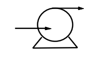
Pumps


Directional arrows showing the flow direction represent a pump (Picture 7).


Picture 7: Pumps


Piping and Connections


Piping and connections are represented with several different symbols (Picture 8):

❑ A heavy solid line represents piping;
❑ A thin solid line represents process connections to instruments (e.g., impulse piping);
❑ A dashed line represents electrical signals (e.g., 4–20 mA connections);
❑ A slashed line represents pneumatic signal tubes;
❑ A line with circles on it represents data links.

Other connection symbols include capillary tubing for filled systems (e.g., remote diaphragm seals), hydraulic signal lines, and guided electromagnetic or sonic signals.


Picture 8: Piping and Connection Symbols


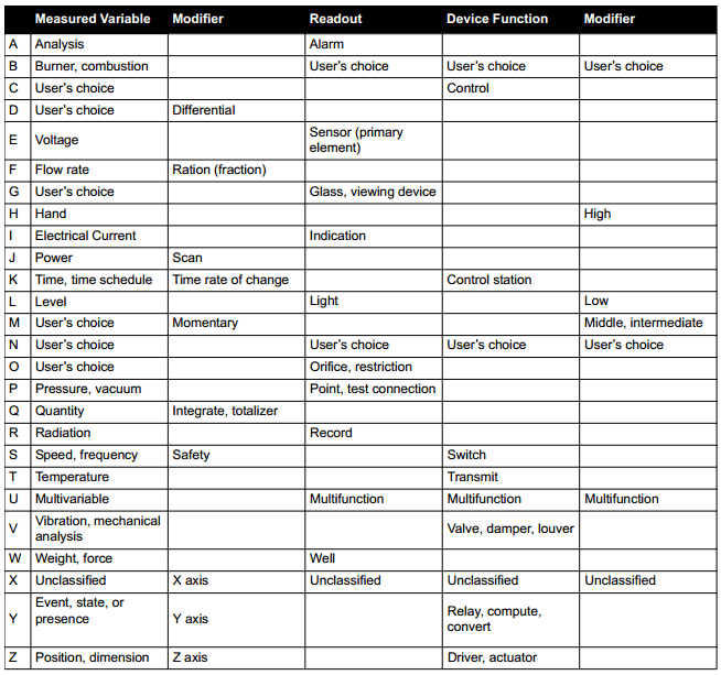
Identification Letters


Identification letters on the ISA symbols (e.g., TT for temperature transmitter) indicate:

❑ The variable being measured (e.g., flow, pressure, temperature);
❑ The device’s function (e.g., transmitter, switch, valve, sensor, indicator);
❑ Some modifiers (e.g., high, low, multifunction).

The table on Picture 9, shows the ISA identification letter designations.

The initial letter indicates the measured variable. The second letter indicates a modifier, readout, or device function. The third letter usually indicates either a device function or a modifier. For example, “FIC” on an instrument tag represents a flow indicating controller. “PT” represents a pressure transmitter. You can find identification letter symbology information on the ISA Web site at http://www.isa.org.


Picture 9: ISA Identification Letters


Tag Numbers


Numbers on P&ID symbols represent instrument tag numbers. Often these numbers are associated with a particular control loop (e.g., flow transmitter 123). See Picture 10.


Picture 10: Identification Letters and Tag Number


Components of Control Loops


This article describes the instruments, technologies, and equipment used to develop and maintain process control loops. In addition, this article describes how process control equipment is represented in technical drawings of control loops.

The goal of this article is to be able to:

❑ Describe the basic function of and, where appropriate, the basic method of operation for the following control loop components:
• Primary element/sensor
• Transducer
• Converter
• Transmitter
• Signal
• Indicator
• Recorder
• Controller
• Correcting element/final control element
• Actuator
❑ List examples of each type of control loop component listed above.
❑ State the advantages of 4–20 mA current signals when compared with other types of signals.
❑ List at least three types of final control elements, and for each one:
• Provide a brief explanation of its method of operation;
• Describe its impact on the control loop;
• List common applications in which it is used.
❑ Given a piping and instrumentation drawing (P&ID), correctly label the:
• Instrument symbols (e.g., control valves, pumps, transmitters);
• Location symbols (e.g., local, panel-front);
• Signal type symbols (e.g., pneumatic, electrical).
❑ Accurately interpret instrument letter designations used on P&IDs.


Control Loop Equipment and Technology


Previously, we described the basic elements of control as measurement, comparison, and adjustment. In practice, there are instruments and strategies to accomplish each of these essential tasks. In some cases, a single process control instrument, such as a modern pressure transmitter, may perform more than one of the basic control functions. Other technologies have been developed so that communication can occur among the components that measure, compare, and adjust.


Primary Elements - Sensors


In all cases, some kind of instrument is measuring changes in the process and reporting a process variable measurement. Some of the greatest ingenuity in the process control field is apparent in sensing devices. Because sensing devices are the first element in the control loop to measure the process variable, they are also called primary elements. Examples of primary elements include:

❑ Pressure sensing diaphragms, strain gauges, capacitance cells;
❑ Resistance temperature detectors (RTDs);
❑ Thermocouples;
❑ Orifice plates;
❑ Pitot tubes;
❑ Venturi tubes;
❑ Magnetic flow tubes;
❑ Coriolis flow tubes;
❑ Radar emitters and receivers;
❑ Ultrasonic emitters and receivers;
❑ Annubar flow elements;
❑ Vortex sheddar.

Primary elements are devices that cause some change in their property with changes in process fluid conditions that can then be measured. For example, when a conductive fluid passes through the magnetic field in a magnetic flow tube, the fluid generates a voltage that is directly proportional to the velocity of the process fluid. The primary element (magnetic flow tube) outputs a voltage that can be measured and used to calculate the fluid’s flow rate. With an RTD, as the temperature of a process fluid surrounding the RTD rises or falls, the electrical resistance of the RTD increases or decreases a proportional amount. The resistance is measured, and from this measurement, temperature is determined.


Transducers and Converters


A transducer is a device that translates a mechanical signal into an electrical signal. For example, inside a capacitance pressure device, a transducer converts changes in pressure into a proportional change in capacitance.

A converter is a device that converts one type of signal into another type of signal. For example, a converter may convert current into voltage or an analog signal into a digital signal. In process control, a converter used to convert a 4–20 mA current signal into a 3–15 psig pneumatic signal (commonly used by valve actuators) is called a current-to-pressure converter.


Transmitters


A transmitter is a device that converts a reading from a sensor or transducer into a standard signal and transmits that signal to a monitor or controller. Transmitter types include:

❑ Pressure transmitters;
❑ Flow transmitters;
❑ Temperature transmitters;
❑ Level transmitters;
❑ Analytic (O2 [oxygen], CO [carbon monoxide], and pH) transmitters.


Signals


There are three kinds of signals that exist for the process industry to transmit the process variable measurement from the instrument to a centralized control system:

1. Pneumatic signal
2. Analog signal
3. Digital signal


Pneumatic Signals


Pneumatic signals are signals produced by changing the air pressure in a signal pipe in proportion to the measured change in a process variable. The common industry standard pneumatic signal range is 3–15 psig. The 3 corresponds to the lower range value (LRV) and the 15 corresponds to the upper range value (URV). Pneumatic signalling is still common. However, since the advent of electronic instruments in the 1960s, the lower costs involved in running electrical signal wire through a plant as opposed to running pressurized air tubes has made pneumatic signal technology less attractive.


Analog Signals


The most common standard electrical signal is the 4–20 mA current signal. With this signal, a transmitter sends a small current through a set of wires. The current signal is a kind of gauge in which 4 mA represents the lowest possible measurement, or zero, and 20 mA represents the highest possible measurement. For example, imagine a process that must be maintained at 100 °C. An RTD temperature sensor and transmitter are installed in the process vessel, and the transmitter is set to produce a 4 mA signal when the process temperature is at 95 °C and a 20 mA signal when the process temperature is at 105 °C. The transmitter will transmit a 12 mA signal when the temperature is at the 100 °C setpoint. As the sensor’s resistance property changes in response to changes in temperature, the transmitter outputs a 4–20 mA signal that is proportionate to the temperature changes. This signal can be converted to a temperature reading or an input to a control device, such as a burner fuel valve. Other common standard electrical signals include the 1–5 V (volts) signal and the pulse output.


Digital Signals


Digital signals are the most recent addition to process control signal technology. Digital signals are discrete levels or values that are combined in specific ways to represent process variables and also carry other information, such as diagnostic information. The methodology used to combine the digital signals is referred to as protocol.
Manufacturers may use either an open or a proprietary digital protocol. Open protocols are those that anyone who is developing a control device can use. Proprietary protocols are owned by specific companies and may be used only with their permission. Open digital protocols include the HART® (highway addressable remote transducer) protocol, FOUNDATION™ Fieldbus, Profibus, DeviceNet, and the Modbus® protocol.


Indicators


While most instruments are connected to a control system, operators sometimes need to check a measurement on the factory floor at the measurement point. An indicator makes this reading possible. An indicator is a human-readable device that displays information about the process. Indicators may be as simple as a pressure or temperature gauge or more complex, such as a digital read-out device. Some indicators simply display the measured variable, while others have control buttons that enable operators to change settings in the field.


Recorders


A recorder is a device that records the output of a measurement devices. Many process manufacturers are required by law to provide a process history to regulatory agencies, and manufacturers use recorders to help meet these regulatory requirements. In addition, manufacturers often use recorders to gather data for trend analyses. By recording the readings of critical measurement points and comparing those readings over time with the results of the process, the process can be improved. Different recorders display the data they collect differently. Some recorders list a set of readings and the times the readings were taken; others create a chart or graph of the readings. Recorders that create charts or graphs are called chart recorders.


Controllers


A controller is a device that receives data from a measurement instrument, compares that data to a programmed setpoint, and, if necessary, signals a control element to take corrective action. Local controllers are usually one of the three types: pneumatic, electronic or programmable. Contollers also commonly reside in a digital control system (Picture 1).


Picture 1: Controllers


Controllers may perform complex mathematical functions to compare a set of data to setpoint or they may perform simple addition or subtraction functions to make comparisons. Controllers always have an ability to receive input, to perform a mathematical function with the input, and to produce an output signal. Common examples of controllers include:

❑ Programmable logic controllers (PLCs)—PLCs are usually computers connected to a set of input/output (I/O) devices. The computers are programmed to respond to inputs by sending outputs to maintain all processes at setpoint.
❑ Distributed control systems (DCSs)—DCSs are controllers that, in addition to performing control functions, provide readings of the status of the process, maintain databases and advanced man-machine-interface.


Correcting Elements - Final Control Elements


The correcting or final control element is the part of the control system that acts to physically change the manipulated variable. In most cases, the final control element is a valve used to restrict or cut off fluid flow, but pump motors, louvers (typically used to regulate air flow), solenoids, and other devices can also be final control elements.
Final control elements are typically used to increase or decrease fluid flow. For example, a final control element may regulate the flow of fuel to a burner to control temperature, the flow of a catalyst into a reactor to control a chemical reaction, or the flow of air into a boiler to control boiler combustion. In any control loop, the speed with which a final control element reacts to correct a variable that is out of setpoint is very important. Many of the technological improvements in final control elements are related to improving their response time.


Actuators


An actuator is the part of a final control device that causes a physical change in the final control device when signalled to do so. The most common example of an actuator is a valve actuator, which opens or closes a valve in response to control signals from a controller. Actuators are often powered pneumatically, hydraulically, or electrically. Diaphragms, bellows, springs, gears, hydraulic pilot valves, pistons, or electric motors are often parts of an actuator system.


Basic Terminology in Closed-loop Control


In Closed and Open Control Loops we look at the difference between open-loop and closed-loop control using the example of volumetric flow for a control valve. In addition we look at the basic principle of closed-loop control and basic terminology. Using this example, let’s take a closer look at closed-loop control terminology.


Controlled variable x


The aim of any closed-loop control is to maintain a variable at a desired value or on a desired-value curve. The variable to be controlled is known as the controlled variable x. In our example it is the volumetric flow.


Manipulated variable y


Automatic closed-loop control can only take place if the machine or system offers a possibility for influencing the controlled variable. The variable which can be changed to influence the controlled variable is called the manipulated variable y. In our example of volumetric flow, the manipulated variable is the drive current for the positioning solenoid.


Disturbance variable z


Disturbances occur in any controlled system. Indeed, disturbances are often the reason why a closed-loop control is required. In our example, the applied pressure changes the volumetric flow and thus requires a change in the control valve setting. Such influences are called disturbance variables z.
The controlled system is the part of a controlled machine or plant in which the controlled variable is to be maintained at the value of the reference variable. The controlled system can be represented as a system with the controlled variable as the output variable and the manipulated variable as the input variable. In the example of the volumetric flow control, the pipe system through which gas flows and the control valve formed the control system.


Reference variable w


The reference variable is also known as the set point. It represents the desired value of the controlled variable. The reference variable can be constant or may vary with time. The instantaneous real value of the controlled variable is called the actual value w.


Deviation xd


The result of a comparison of reference variable and controlled variable is the deviation xd:

xd = w - x


Control response


Control response indicates how the controlled system reacts to changes to the input variable. Determination of the control response is one of the aims of closed-loop control technology.


Controller


The controller has the task of holding the controlled variable as near as possible to the reference variable. The controller constantly compares the value of the controlled variable with the value of the reference variable. From this comparison and the control response, the controller determines and changes the value of the manipulating variable (see Picture 1).


Picture 1: Functional principle of a closed-loop control


Manipulating element and servo-drive


The manipulating element adjusts the controlled variable. The manipulating element is normally actuated by a special servo drive. A servo drive is required if it is not possible for the controller to actuate the manipulating element directly. In our example of volumetric flow control, the manipulating element is the control valve.


Measuring element


In order to make the controlled variable accessible to the controller, it must be measured by a measuring element (sensor, transducer) and converted into a physical variable that can be processed by the controller is an input.


Closed loop


The closed loop contains all components necessary for automatic closed-loop control (see Picture 2).


Picture 2: Block diagram of a control loop